Computational Muddles
There is a reason I liken computations to evanescent spirits. They are called into being with obscure incantations, spin filaments of data into complex webs of information, and then vanish with little trace of their ephemeral calculations. Of course, there are observable side effects, say when a computation activates a physical device or causes output to be sent to a printer, displayed on a screen or stored in a file. But the computations themselves are difficult to observe in much the way your thoughts are difficult to observe.
I’m exaggerating somewhat; after all, unlike our brains, computers are designed by human beings. We can trace every signal and change that occurs in a computer. The problem is that a complete description of all those signals and changes does not help much in understanding what’s going on during a complex computation; in particular, it doesn’t help figure out what went wrong when the results of a computation don’t match our expectations.
An abstraction is a way of thinking about problems or complex phenomena that ignores some aspects in order to simplify thinking about others. The idea of a digital computer is itself an abstraction. The computers we work with are electrical devices whose circuits propagate continuously varying signals; they don’t operate with discrete integers 0, 1, 2, ..., or for that matter with binary digits 0 and 1. The idea that computers deal with 1s and 0s is an abstraction.
The dependability of this abstraction is a testimony to the many electrical engineers and physicists who developed modern computers. It would complicate things considerably if every once in a while when you add 1 and 0 you got something a little more, say 1.0012, or a little less, say 0.99998, than 1. If you’re a digital circuit designer, you can never forget that the signals in computer circuits are continuous; your job is to make them behave according to the digital abstraction. As a programmer you can safely adopt the digital abstraction, but you’ll need additional abstractions to develop sophisticated software.
5.1 Computational models
The term computational modelis often used to describe an abstraction that simplifies thinking about computation. Chapter 1’s abstraction of Unix pipes passing information between commands in shell scripts is a computational model. The metaphor of files as fluid flowing continuously through pipes is potentially misleading. However, we can easily weave a somewhat more complicated story around the pipe abstraction to provide a more accurate picture of what’s going on during the execution of a shell script.
Think of each command in a shell script as a bureaucrat responsible for some particular paper-shuffling task in a company. Imagine that the bureaucrats are linked to one another via a set of pneumatic tubes of the sort found in 19th-century factories and office buildings. To send a purchase order to the fellow in accounting for approval, you put it in a little capsule and stuff it in the right tube; the capsule is sucked through the system and ends up on the desk of the fellow in accounting in a matter of seconds. The messages thus zip through these pneumatic tubes and land on the desk of one bureaucrat who processes each message in the order in which it arrived and then sends it along to the next bureaucrat by placing it into his outgoing pneumatic tube. A little quaint, perhaps, but easy to visualize and it does a pretty good job of describing reality. With this abstraction, we move from plumbing pipes carrying some sort of fluid (a continuous view of the world) to pneumatic tubes carrying individual messages (a discrete view of the world).
As we move from one-line shell scripts composed of powerful commands whose inner workings we largely ignore to programs consisting of many lines and involving components of considerable complexity whose inner workings we have to comprehend and in many cases design, we need more powerful computational models. But just because these models are more powerful doesn’t mean they have to be more complex. In this chapter we’ll be looking at some relatively simple models that can be used to understand a broad range of computations. We’ll be going back over some of the territory we covered in Chapter 4 but this time with different objectives in mind.
I’ve heard some computer scientists say that the most important prerequisite for learning how to program is knowing a little algebra. While this is largely true, it is rarely a comfort to students thinking of taking a computer science class. Many people found learning algebra painful, all the more so because it wouldn’t go away — you needed it for all sorts of other things. Fortunately, the kind of algebra required to carry out basic programming tasks is of a particularly benign sort. Those of you who aced algebra, however: don’t get too excited, because being good at algebra is not the only skill you need to become a good computer scientist or programmer.
|
To follow the connection from algebra to programming, consider this simple word problem like those you met in grade school:
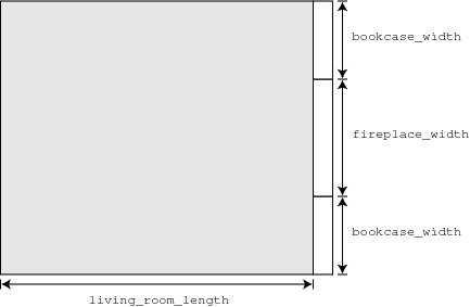
Anne wants to buy carpeting to cover her living-room floor. The room is rectangular and 8 meters long. At one end of the room, there is a 3-meter-wide fireplace flanked by two identical bookcases that, together with the fireplace, take up the entire width of the room. The bookcases are 2 meters wide each. The fireplace and two bookcases are built into the wall and don’t cover any of the floor space. The carpeting Anne wants costs $5 per square meter. How much will Anne have to pay for her new carpet?
How would you solve this problem? I usually start by drawing a diagram like the one in Figure 6; we want to calculate the shaded area. Next you’ll have to recall the mathematical relationship involving area and the dimensions (length and width) of a rectangle. Algebraically, you would write this down as a formula involving three variables or terms that we specify using easily remembered (mnemonic) names:
living_room_area = living_room_length * living_room_width
Following a convention common in programming languages, the * here stands for multiplication. For simplicity, all the terms in our formulas will be unitless, which means we’ll have to be careful not to add a term specified in meters to one specified in kilometers.
You’d also write down the the specified quantities and relationships in the word problem, introducing additional terms as needed:
living_room_length = 8

bookcase_width = 2

fireplace_width = 3

cost_per_square_meter = 5

living_room_width = fireplace_width + (2 * bookcase_width)
and the formula for answering the question posed:
total_cost = cost_per_square_meter * living_room_area
Now to calculate the answer, you just “plug and chug”, as engineering students like to say. Starting with the basic formula
total_cost = cost_per_square_meter * living_room_area
you proceed by substituting (the “plug” part) the appropriate formulas and values for the terms in the formula and simplifying (the “chug” part) by performing arithmetic operations (addition, subtraction, multiplication) as appropriate:
total_cost = cost_per_square_meter *
             living_room_length * living_room_width

total_cost = cost_per_square_meter *
             living_room_length *
             (fireplace_width + (2 * bookcase_width))

total_cost = cost_per_square_meter *
             living_room_length * (fireplace_width + (2 * 2)))

total_cost = cost_per_square_meter *
             (living_room_length * (fireplace_width + 4))

total_cost = cost_per_square_meter * (living_room_length * (3 + 4))

total_cost = cost_per_square_meter * (living_room_length * 7)

total_cost = cost_per_square_meter * (8 * 7)

total_cost = cost_per_square_meter * 56

total_cost = 5 * 56

total_cost = 280
Note how our original formula
total_cost = cost_per_square_meter * living_room_area
expanded and contracted as we made substitutions and simplified subformulas.
In a language like Scheme, we’d specify the entities and relationships much as we did here, though we’d have to adhere to Scheme’s syntax, which takes a little getting used to. In Scheme, an expression like
(define living_room_length 8)
tells the Scheme interpreter that we are definingthe term living_room_length to be 8. If we subsequently ask Scheme to “evaluate” living_room_length, it looks up this definition and returns the “value” 8. Here’s what interacting with the Scheme interpreter looks like:
> (define living_room_length 8)
> living_room_length
8
The first typed expression was interpreted as a request to make the indicated definition; Scheme had nothing to say about this so the prompt immediately reappeared. The second typed expression was interpreted as a request to “evaluate” the expression, which Scheme did by printing out the result. (This form of interaction is called a “read, evaluate and print loop” for obvious reasons.) We can continue to define the other terms in our word problem:
> (define bookcase_width  2)
> (define fireplace_width 3)
> (define cost_per_square_meter 5)
> (define living_room_width (+ fireplace_width (* 2 bookcase_width)))
The last line is bit different: The definition is a compound expression that involves previously defined terms as well as mathematical operators in Polish notation(operators precede their arguments). When Scheme sees an expression of this compound form, it evaluates it by replacing the values of the terms in the expression with their values as defined previously and then simplifying to obtain a value to use as the definition of the new term, living_room_width here. If we submit this term to the interpreter now, it looks up the newly minted definition, as you might expect:
> living_room_width
7
The next definition is a very different animal:
> (define (total_cost unit_cost quantity) (* unit_cost quantity))
Scheme behaves very differently when it encounters an attempt to define an expression of the form (some-term args), where some-term is a placeholder for the name of a “function”(also called a “procedure”) and args is a placeholder for one or more terms called “formal parameters”(also called the “arguments”to the function). Unlike the earlier definition in which Scheme evaluated the compound expression, when a function is defined, Scheme stores both the calling pattern, here (total_cost unit_cost quantity), and the function definition, (* unit_cost quantity). It doesn’t evaluate the function definition as it did expression in a definition of the form (define name expression). A definition of the form (define (name args) expression) is special in that it provides a general recipe for performing a computation, a recipe that is carried out whenever Scheme is asked to evaluate an expression of the form (name args).
We use this form of definition again to specify one last formula:
> (define (living_room_area width length) (* width length))
Now that we’ve defined all of the relevant terms and formulas, we can ask Scheme to evaluate an expression corresponding to the answer to the word problem:
> (total_cost cost_per_square_meter
              (living_room_area living_room_width
                                living_room_length))
280
Here are the steps Scheme takes to evaluate this expression:
(total_cost cost_per_square_meter
            (living_room_area living_room_width
                              living_room_length))
(total_cost 5
            (living_room_area living_room_width
                              living_room_length))
(total_cost 5
            (living_room_area 7
                              living_room_length))
(total_cost 5 (living_room_area 7 8))
(total_cost 5 (* 7 8))
(total_cost 5 56)
(* 5 56)
280
To be more precise, this is just one possible sequence of steps that a Scheme interpreter might take in order to evaluate the expression. In writing code for a Scheme interpreter, a programmer has two primary goals: first, to make sure that the interpreter evaluates expressions according to the semantics of the language and second, to make sure that those evaluations are done quickly. The semanticsof a language specifies the meaning of expressions formed in accord with the syntax of that language. Scheme has a formal and an informal (intuitive) semantics and I’ll rely entirely on the latter in this chapter. As with a spoken or natural language, an intuitive semantics for a programming language explains the meaning of more complex expressions in terms of the meaning of simpler ones; for example, the meaning of (+ 1 2) is 3. In general, we’ll use our understanding of arithmetic and algebra in deciphering the meaning of Scheme expressions.
As an alternative to our first specification and to make the Scheme calculations look a little more like our algebraic manipulations, we can define a special-purpose function to replace our previous definition of living_room_width:
> (define (living_room_width bookcase_width fireplace_width)
      (+ fireplace_width (* 2 bookcase_width)))
In defining this function, as in invoking total_cost, we used more than one line. When functions become longer and more complicated, programmers use indentation and formatting to keep track of arguments and nested expressions. I often line up arguments vertically, as in this alternative formatting of the living_room_width definition:
> (define (living_room_width bookcase_width fireplace_width)
     (+ fireplace_width
        (* 2
           bookcase_width)))
Formatting is just one way in which programmers try to make code more readable, easier to understand and hence easier to write and modify, both for the original programmer and for other programmers who might want to use or adapt the code later.
5.2 The substitution model
With our new definition for living_room_width, the computation looks more like the algebraic substitutions and simplifications we saw earlier. The model of computation as a sequence of substitutions and simplifications, called the substitution model, is probably the most useful abstraction for thinking about computing. Most programmers, whether they know it or not, use the substitution model every day.
When we first defined living_room_width, we assigned it the number 7, which was the result of a computation. The second time we defined living_room_width we defined it as a function that, when invoked with the proper arguments, computes the width of the living room from a formula (specified in the function definition). Each time living_room_width is invoked with the correct number of arguments, it substitutes the arguments into the formula and evaluates the result.
You may have been puzzled by the fact that the formal parameters to living_room_width have the same names as two terms we defined earlier, bookcase_width and fireplace_width. The whole business of deciphering the meaning of terms and establishing different contexts in which they can have different meanings is important in designing programming languages that can be used to build large programs involving many different programmers. Even a single programmer is likely to use the same term in multiple independent contexts.
The letter “x” must be one of the most frequent variable names in mathematics. In the next exchange, it should be pretty clear what I mean even though I use x twice as a formal parameter, once to assign it a value and once to refer to it as the argument to a function:
> (define (square x) (* x x))
> (define (double x) (+ x x))
> (define x 3)
> (define y (double (square x)))
> y
18
Here’s the new method of calculating the answer to our word program:
> (total_cost cost_per_square_meter
              (living_room_area (living_room_width bookcase_width
                                                   fireplace_width)
                                living_room_length))
280
And here is the series of substitutions and simplifications the Scheme interpreter performed:
(total_cost cost_per_square_meter
            (living_room_area (living_room_width bookcase_width
                                                 fireplace_width)
                              living_room_length))
(total_cost 5
            (living_room_area (living_room_width bookcase_width
                                                 fireplace_width)
                              living_room_length))
(total_cost 5
            (living_room_area (living_room_width 2
                                                 fireplace_width)
                              living_room_length))
(total_cost 5
            (living_room_area (living_room_width 2 3)
                              living_room_length))
(total_cost 5
            (living_room_area (+ 3 (* 2 2))
                              living_room_length))
(total_cost 5
            (living_room_area (+ 3 4) living_room_length))
(total_cost 5 (living_room_area 7 living_room_length))
(total_cost 5 (living_room_area 7 8))
(total_cost 5 (* 7 8))
(total_cost 5 56)
(* 5 56)
280
We can use this same trick of substitution to explain the calculations performed by the factorial function in Chapter 4:
> (define (factorial n) (if (= n 1) 1 (* n (factorial (- n 1)))))
> (factorial 3)
6
Here’s the sequence of substitutions and simplifications; we don’t simplify any subformulas unless we have to:
(factorial 3)
(if (= 3 1) 1 (* 3 (factorial (- 3 1))))
(if #f 1 (* 3 (factorial (- 3 1))))
(* 3 (factorial (- 3 1)))
(* 3 (factorial 2))
(* 3 (if (= 2 1) 1 (* 2 (factorial (- 2 1)))))
(* 3 (if #f 1 (* 2 (factorial (- 2 1)))))
(* 3 (* 2 (factorial (- 2 1))))
(* 3 (* 2 (factorial 1)))
(* 3 (* 2 (if (= 1 1) 1 (* 1 (factorial (- 1 1))))))
(* 3 (* 2 (if #t 1 (* 1 (factorial (- 1 1))))))
(* 3 (* 2 1))
(* 3 2)
6
You may have stumbled over interpreting the expression (if (= 3 1) 1 (factorial (- 3 1))). Scheme interprets this as saying: if 3 is equal to 1 then this expression simplifies to 1, otherwise it simplifies to (factorial (- 3 1)). A so-called “conditional” statement of the form (if test then else), where test, then and else are expressions, is interpreted as follows: if the test expression evaluates to true (#t in Scheme), evaluate the then expression and substitute its value for the conditional statement; but if the test expression evaluates to false (#f in Scheme), don’t mess with the then expression at all but instead evaluate the else expression by substituting its value for the conditional statement. The test statements can be quite complex in general, combining simpler tests using operators such as or and and and not. For example, the expression
(if (and test1 (or test2 (not (test3)))) (+ 1 2) (* 1 2))
evaluates to 3 ((+ 1 2)) if test1 is true and either test2 is true or test3 is false and otherwise to 2 ((* 1 2)).
The exact sequence of substitutions and simplifications used in calculating (factorial 3) is complicated. To take a somewhat closer look, we’ll use a program called a stepperthat walks us through Scheme’s steps in interpreting (factorial 3) (at least when viewed through the abstraction of the substitution model). Here is a sequence of transformations in which each transformation has the form initial expression => resulting expression and the substitutions are highlighted by enclosing the pre- and post-transformation subexpressions in square brackets:
[(factorial 3)] =>
[(if (= 3 1) 1 (* 3 (factorial (- 3 1))))]

(if [(= 3 1)] 1 (* 3 (factorial (- 3 1)))) =>
(if [#f] 1 (* 3 (factorial (- 3 1))))

[(if #f 1 (* 3 (factorial (- 3 1))))] =>
[(* 3 (factorial (- 3 1)))]

(* 3 (factorial [(- 3 1)])) =>
(* 3 (factorial [2]))

(* 3 [(factorial 2)]) =>
(* 3 [(if (= 2 1) 1 (* 2 (factorial (- 2 1))))])

(* 3 (if [(= 2 1)] 1 (* 2 (factorial (- 2 1))))) =>
(* 3 (if [#f] 1 (* 2 (factorial (- 2 1)))))

(* 3 [(if #f 1 (* 2 (factorial (- 2 1))))]) =>
(* 3 [(* 2 (factorial (- 2 1)))])

(* 3 (* 2 (factorial [(- 2 1)]))) =>
(* 3 (* 2 (factorial [1])))

(* 3 (* 2 [(factorial 1)])) =>
(* 3 (* 2 [(if (= 1 1) 1 (* 1 (factorial (- 1 1))))]))

(* 3 (* 2 (if [(= 1 1)] 1 (* 1 (factorial (- 1 1)))))) =>
(* 3 (* 2 (if [#t] 1 (* 1 (factorial (- 1 1))))))

(* 3 (* 2 [(if #t 1 (* 1 (factorial (- 1 1))))])) =>
(* 3 (* 2 [1]))

(* 3 [(* 2 1)]) =>
(* 3 [2])

[(* 3 2)] =>
[6]
The stepper gives us a close look at a Scheme computation as seen through the lens of the substitution model. Very few programmers want to look at a complex computation at this level of detail, but in trying to find a problem with program (a process called debugging) they may look this closely at selected parts of a computation. For instance, you could tell the stepper to step through only the transformations for selected functions and summarize all other computations — for example, use [(factorial 3)] => [6] to summarize the computations of the factorial function. As much detail as there is in this sequence of transformations, as much or more is abstracted away; at the level of primitive instructions executed directly by the CPU, the computation involves many more steps than those few shown here.
5.3 Syntax and style revisited
In defining the factorial function, I used a powerful method that sometimes throws students for a loop (pun intended, as you’ll soon discover). The definition of factorial is recursive, meaning that I used factorial to define factorial: the term being defined appears in or “recurs” in the definition.
(define (factorial n)
   (if (= n 1)
       1
       (* n
          (factorial (- n 1)))))
I promise you that this really isn’t a big deal and it seems perfectly natural to lots of students, particularly when they see how it works and aren’t scared off by a teacher who feels recursion is somehow “abnormal.” Some folks think that the “normal” way of computing factorial runs something like this:
int factorial( int n ) {
       int result = 1;
       for ( int i = 2; i <= n; i++ ) {
           result = result * i;
       }
       return result;
}
This is the same syntax for the factorial function that we met at the end of Chapter 4. In prose form, it would read something like: to compute the function n factorial, first assign the variable result to be equal to 1, then begin a loop in which the “iteration” variable i is first set to 2 (i = 2) and then incremented by 1 (i++) on each iteration until i is equal to n; on each iteration in which the body of the loop is executed (those iterations in which i is assigned one of 2, 3, ..., n - 1), reassign the variable result to have its old value times the value of the iteration variable, i. Finally after you’ve completed the loop, return the last assigned value of result.
Asked to calculate factorial(3), this program first sets the variable result to 1, then starts through the “for loop,”setting result to be result times 2 (result is now equal to 2) on the first iteration, and result to be result times 3 (result is now equal to 6) on the second and last iteration, before returning the final value of result, which is 6 in this case. Each time through the loop, the program checks to see if i is greater than 3; if so, it exits the loop without executing the body. In C, the body of a loop is set off with curly brackets { and } following the keyword for and the iteration variable specification ( int i = 2; i <= n; i++ ), so that, in the last definition, the body is just the single statement result = result * i. This is a perfectly good way of calculating factorial and I have no problem whatsoever with it, but the recursive definition is also fine and, to my mind, simple and elegant.
You might worry that a recursive definition would keep calling itself indefinitely, and indeed this is a concern in writing recursive function definitions. The trick is to arrange things so that some argument (assignment to a formal parameter) in the recursive call steadily gets closer to the terminating condition, (= n 1) in the case of factorial. It takes a little practice, but once you get the hang of it, designing recursive definitions with appropriate terminating conditions becomes pretty easy. If you really have an aversion to recursion (or experience some dissonance with assonance), then there are always other languages that are less elegant and less cool ... just kidding; most dialects of Lisp support other methods of iteration besides recursion.
Indeed, Lisp programmers often use the equivalent of C for loops. The Scheme doconstruct is a general iterative construct. When an expression of the form (do (var-init-step-expressions) (test exit) body) is evaluated, each variable mentioned in the list of var-init-step expressions is bound to the result of evaluating the variable’s corresponding init expression, then the termination condition test is evaluated. If the termination condition evaluates to true (#t), then any exit expressions are evaluated. If the termination condition evaluates to false (#f), then the expressions in the body are evaluated. On each subsequent iteration, each of the variables is updated using its corresponding step expression if present. The Scheme expression (do ((i 1 (+ i 1))) ((= i n)) body) is essentially equivalent to for (int i = 1; i < n; i++) { body } in C or Java.
Here’s a translation of the “normal” implementation of factorial to Scheme using do:
(define (factorial n)
  (let ((result 1))
    (do ((i 2 (+ i 1)))
        ((> i n) result)
      (set! result (* result i)))))
We won’t explore let (it’s used to introduce local variables) or set! (it’s an assignment operator) until the next chapter, but you should have a pretty good idea of how this implementation works. You may prefer this to the recursive definition; however, it’s worthwhile becoming comfortable with both styles, as you’re likely to encounter both in reading code.
While we’re on the subject of preferences, if you went off and got a programming job today, you’d probably end up using Java, C, C++, various web-page formatting languages like HTML and various scripting languages like JavaScript, Perl and PHP. In a couple of years, perhaps C#, Python and XHTML will be the hot languages to know. At this stage, though, don’t worry too much about which language to program in, just learn to program and have some fun at it. If you end up programming for your own professional or recreational purposes, almost any language with a reasonably large and dedicated following will do just fine. And if you learn to program well, picking up a new language will be relatively easy.
By the way, the substitution model works fine for understanding any program written in any programming language. However, to have a completely general model, we’d need to extend the model to handle assignments, for example, i = 1 in Java or C and set! in Scheme, loops and other flow-of-control mechanisms. We’d also have to extend it to handle programming concepts like object-oriented programming. Discussing these extensions would take us too far afield from my aim of giving you a high-level overview of interesting computational ideas. So let’s leave the substitution model behind and explore some different computational models, including some that lead us to an object-oriented view of programming.