Searching the Wild Web
The technology supporting the World Wide Web enables computations and data to be distributed over networks of computers, and this lets you use programs that you don’t have to install or maintain and gain access to information that you don’t have store or worry about backing up. The World Wide Web is essentially a global computer with a world-wide file system.
Many of the documents in this huge file system are accessible to anyone with a browser and a network connection. Indeed, their authors really want you to take a look at what they have to offer in the terms of advice, information, merchandise and services. Some of these documents, we tell ourselves, contain exactly what we’re looking for, but it isn’t always easy to find them.
It’s difficult enough to search through files full of your own personal stuff — now there are billions of files generated by millions of authors. Some of those authors are likely to be somewhat misleading in promoting whatever they’re offering, others may be downright devious, and some will just be clueless, ignorant about whatever they’re talking about. How can we sift through this morass of data and find what we’re looking for?
14.1 Spiders in the web
Billions of files are stored on web servers all over the world and you don’t need a browser to access them. Programmers typically use libraries implementing the HTTPand FTPprotocols to grab files off the web. We’ll continue to use a shell for our investigations and, not surprisingly, there are all sorts of programs for exploring the web that can be easily invoked from a shell. curl is a popular utility program supporting several protocols to transfer files specified as URLs. Here I use curl to grab an HTML file sitting in the directory on the Brown web server that stores my web pages:
% curl www.cs.brown.edu/people/tld/file.html
<HTML>
<HEAD>
<TITLE>Simple HTML File</TITLE>
</HEAD>
<BODY>
<H1>Section Heading</H1>
<P>
Here is a file containing HTML formatting
commands that has a body consisting of
one section heading and a single paragraph.
</P>
</BODY>
</HTML>
Perhaps you’ve seen files containing HTML commands before. This file is very simple HTML code and I expect you can figure out the basic idea. Sometimes the HTML formatting can be useful in searching files on the web, but for our purposes it’ll just get in the way. I could pipe the output of curlinto an HTML-to-text converter, but I can’t find a converter on this machine and I’m lazy so I’m going to take a shortcut. Your web browser interprets (or parses) HTML formatting commands and then displays the results in a graphics window using all sorts of pretty fonts and images. I’m going to use a text-based (no graphics, no fancy on-screen formatting) browser called lynx to parse HTML files and strip away all the formatting commands so I can manipulate the raw text. lynx is a very useful tool to add to your bag of tricks: you can use it to surf the web, but I use it here just to dump the text — minus the HTML formatting — to a shell or to a file with the -dump option and the -nolist option, which suppresses any information about hyperlinks found in the HTML file:
% lynx -dump -nolist www.cs.brown.edu/people/tld/file.html

   Section Heading

   Here is a file containing HTML formatting
   commands that has a body consisting of
   one section heading and a single paragraph.
There is still a bit of formatting (spaces and line breaks) in the text-based output, but I can filter that out by removing the extraneous white space. The important point is that I can now treat the web as a huge repository of text files. These files aren’t stored in a single hierarchical directory like my personal files; they are located on machines all over the world. But even if I had the time and the storage space, how could I ever download all the files on the web? And why would I ever want to?
The answer to the second question is easy. You can’t know for sure whether a file contains what you’re looking for unless you, or your computer-animated proxy, at least look at it, and, in order to look at a file, you have to download it to your machine. As for how you’d download all the files on the web — at least in principle, you’d do so by following hyperlinks. While the details can get pretty complicated, the basic algorithm is simple.
Start with one or more URLs. For each URL, use curl or some other HTTP-savvy program to download the file and store it in an appropriately named file (in theory, URLs are unique, so a file name based on the URL is a good starting point; in practice, you have to work harder to find a unique name). Next use an HTML parser like the one in lynx to extract all the URLs corresponding to hyperlinks in the file and add these to your set of URLs to download. (Be sure to eliminate any URLs you’ve already downloaded, otherwise you may get into an infinite loop, loading the same files over and over again.1) Now just settle down and wait for your algorithm to terminate.
As they say, “don’t try this at home.” It would take you a very long time to traverse the entire web, and even if you were to strip off all the JPEG and GIF image files and all the MP3 music files and just store the raw text, you’d still end up with a lot more data than you could possibly handle. But that’s not to say it isn’t done. Companies that provide content searches on the web (so-called search-enginecompanies) like Google, AltaVista, Lycos, and others employ thousands of computers arranged in huge server farmsto constantly scour the web in order to maintain as accurate an account of the files on the web as is technologically feasible. These server farms together with the software that runs on them, variously called crawlers, trawlers, bots and spiders, reduce searching the web to searching through a set of files, albeit a very large set of files.
So why can’t we just use grepagain? Part of the problem is that a simple keyword search, like looking for all files containing the words Javaand Scheme, is likely to include lots of irrelevant files. In addition to finding files that only casually mention Java and Scheme, you’re likely to find files concerned with decorating plans involving shades of brown, coffee cultivation strategies and Indonesian politics. We could pay a lot of people to read the files and then index them and even rank their relevance (indeed, some search-engine companies do exactly that). But we’re lazy (and impatient), and besides it’s a losing battle with thousands if not millions of new web pages being produced every day. How can we automate finding relevant files and ranking their importance? How do we find the really good stuff?
14.2 Measuring similarity
We don’t yet have programs that can read and understand prose, but the field of information retrievalhas discovered some useful tricks for searching large archives (called corpora) of text documents. As far as our linguistically challenged programs are concerned, a file is just a bag full of words with some formatting that may or may not be relevant. Some of the words are probably meaningful, such as those that appear in few files, and others aren’t particularly useful, such as words like “a”, “the” and “of” that appear frequently in almost every file. If the word appears in only a few files, then the number of times it appears in a file may provide additional information; files containing information about Java will probably include several occurrences of the word “Java.”
Let’s take a look at some actual data. Here are the URLs of nine web pages, including three pages concerned with the Java programming language, three about HTML and the World Wide Web and three that have something to do with Scheme (the terms on the right will be used to refer to the URLs in tables and graphs):
java.sun.com          Sun Microsystems Java          java
www.javalobby.org     Java Discussion Forums         lobby
www.javaworld.com     Java News and Information      world
www.w3.org            World Wide Web Consortium      www
www.hwg.org           The HTML Writers Guild         guild
www.htmlgoodies.com   HTML Tools and Resources       html
www.scheme.org        Information about Scheme       scheme
www.drscheme.org      An Implementation of Scheme    doctor
www.schemers.com      Scheme Educational Software    edsoft
I want to look at the frequency of the words in some of these files. A word histogramfor a file gives each word in the file along with the total number of times the word appears. The following interaction with the shell lists a short Perlprogram2 that counts the number of occurrences of each word in a file and then prints out the file’s histogram.
% cat tf.pl
#!/usr/bin/perl
while ($_ = <ARGV>) {
    tr/A-Z/a-z/;
    @words = split(/\W+/, $_);
    foreach $word (@words) {
        $wordcount{$word}++;
    }
}
sub bycount {
    $wordcount{$a} <=> $wordcount{$b};
}
foreach $word (sort bycount keys ( %wordcount )) {
    printf "%10s %d\n", $word, $wordcount{$word};
}
You can get the gist without understanding every particular, but it helps to know that tr converts characters to lower case, split breaks a line of text into a list of the words appearing in the line, and wordcount is a list of pairs each consisting of a key (a word in this case) and an integer that keeps a running count of the number of occurrences of each word. In the terminology of Chapter 13, wordcount is an association list and $wordcount{$word} returns the value associated with the word corresponding to $word, the count of the number of occurrences of the word. $wordcount{$word}++ is convenient shorthand syntax for incrementing the count associated with the word corresponding to $word.
We’ll use this little program to display part of the word histogram for the JavaWorld web page:
% lynx -dump -nolist www.javaworld.com | perl tf.pl | tail
 javaworld 9
      from 9
       for 9
       net 10
        of 10
         a 12
        to 13
       and 19
       the 23
      java 28
I used tail to list only the ten (the default value for tail) most frequently appearing words in the file. Using simple variations on this script, I determined that the JavaWorld file contains 605 words of which 339 are distinct. Commonly used words (called stop wordsin information-retrieval parlance) and topic-related words appear the most often in the text. The only way to distinguish stop words from topic-related words is to have some idea of the frequency with which the words appear in all files.
Let’s take a look at the HTML Writers Guild web page:
% lynx -dump -nolist www.hwg.org | perl tf.pl | tail
    online 5
    member 5
      html 7
       for 7
       web 9
        to 10
        in 10
       and 11
     guild 13
       the 25
The word “java” doesn’t appear (at least in the top 10) but the words “html”, “web” and “guild” do. In this case there are only 345 words of which 200 are unique. So, what information can we easily extract from the text file that our programs see as a bag of words? There is the set of words, their respective word counts and the total number of words. In addition, by looking at the entire collection of files (the corpus), we can determine the frequency with which a word appears in any file, thereby obtaining some insight on how common it is. We want to summarize each file by stripping off the information we can’t use and emphasizing the information that we can. As a first step, I’ll run a little shell script that reads each test file and then prints summaries to a data file tf.dat. This shell script is written in the scripting language for the C shell (csh), which looks a lot like Perl or C. Here’s how to parse it.
The first line, #!/bin/csh, indicates that this script should be run using the C shell program, csh. The statement if ( -r tf.dat ) /bin/rm tf.dat removes (using the rm command) the old file tf.dat if one is present in the current directory. The touch tf.dat line creates a new empty file of the same name. The variable urls is assigned to be the list of all the URLs for the web pages we want to process. Finally, the foreach statement processes each URL and appends the resulting information to the file tf.dat using the >> redirection operator.
% cat tf.csh
#!/bin/csh
if ( -r tf.dat ) /bin/rm tf.dat
touch tf.dat
set urls=(java.sun.com\
          www.javaworld.com\
          www.javalobby.org\
          www.scheme.org\
          www.schemers.com\
          www.drscheme.org\
          www.w3.org\
          www.htmlgoodies.com\
          www.hwg.org)
foreach url ( $urls )
        printf "(%s" $url >> tf.dat
        lynx -dump -nolist $url | perl tf.pl >> tf.dat
        printf ")" >> tf.dat
        end
% csh tf.csh
In brief, this script specifies a list of URLs and then uses a little loop to invoke lynx and the word-histogram Perl script on each URL. The result of executing this script is a file, tf.dat, comprised of lists (note the printf statements that bracket each call to lynx) consisting of a URL followed by word/count pairs.
Why did I do this? I wanted to convert the URLs to summaries of the information in their respective files and I wanted the summaries in a format that I could easily use in a Scheme program to manipulate the data further. Shell and Perl scripts are wonderful tools for managing files but I prefer languages like C, Java and Scheme for more complicated computations, partly from habit and partly because high-level languages like Java and Scheme in particular are designed to encourage good programming habits. The summaries in tf.dat are now in a form that I can easily read from Scheme. I’m not going to list the entire Scheme program (you can download it from www.cs.brown.edu/people/tld/talk/ if you’re interested in looking at it, running it or modifying it for your own purposes). Here’s what my Scheme program does with the summaries.
First, it scans all the summaries and creates a list of all the words in any file3. There are 1492 distinct words appearing in the nine files. The program assigns to each word an integer between 1 and 1492 called its index. Then for each file corresponding to a URL, the program creates a list (called a vector) in which the ith item is the number of times the word with index i appears in the file. Many items in the vector for a given file are likely to be 0 since many of the 1492 words appear in only one file. If the indices for the words “and”,“the” and “java” are 1, 2 and 3, respectively, then the vector for JavaWorld is (19 23 28 ...) and the vector for the HTML Writers Guild is (11 25 0 ...). These vectors, with their consistent method of using indices referring to word counts, will replace the original summaries.
How might we analyze two such vectors to determine if the corresponding two files are similar? Information-retrieval experts use mathematical tools from linear algebra and probability theory to measure similarity, but there are simpler expedients that do a pretty good job. Most methods operate by combining differences at the word level. For example, take the sum of the absolute values of the differences of the word counts: then the similarity of the JavaWorld and HTML Writers Guild web pages would be measured by (+ (abs (- 19 11)) (abs (- 23 25)) (abs (- 28 0)) ...), or (+ 8 2 28 ...). You could take the square of the difference of the word counts and you’d get a measure related to Euclidean distance, albeit in a geometry of 1492 dimensions instead of the usual three.4 With a few optimizations, variations on these basic ideas turn out to work well in practice.
My little Scheme program uses some standard tricks from information retrieval. Instead of the raw word counts, my program uses the term frequencyfor each word, defined as the number of times the word appears in the file divided by the total number of words in the file. By using (19/605 23/605 28/605 ...) and (11/345 25/345 0/345 ...) instead of (19 23 28 ...) and (11 25 0 ...) for the JavaWorld and HTML Writers Guild vectors, we adjust the word counts to reflect different file sizes — (- 19/605 11/345) is tiny compared to (- 19 11). The term frequencies are further adjusted by weighting them by some function of the inverse document frequency, the total number of files divided by the number of files in which the word appears. This adjustment deemphasizes differences based on commonly occurring words.
Finally, instead of using a sum of absolute differences, my program treats each vector as a line through the origin of a 1492-dimensional vector space (linear algebra jargon) and computes the cosine of the angle between the vectors as the measure of similarity. Suffice it to say that this cosine method is easy to compute, makes perfect sense to someone who is comfortable maneuvering in super-high-dimensional vector spaces and yields a measure that ranges from 1, very similar, to 0, not similar at all. When I load my Scheme code it automatically reads in the data in tf.dat and computes the vectors for the nine test files:
% scheme
> (load "tf.scm")
The file tf.scm contains about a hundred or so lines of code, most of which handles cleaning up the data and creating and comparing vectors. In particular, this file defines a Scheme function that takes a string specifying a URL and uses the cosine method to compare the vector for the corresponding file with the vectors for the other files. It then prints out each of the nine test URLs preceded by the result computed with the cosine method:
> (compare "www.w3.org")
1.000 www.w3.org
0.098 www.hwg.org
0.075 www.htmlgoodies.com
0.070 java.sun.com
0.063 www.javalobby.org
0.053 www.javaworld.com
0.045 www.schemers.com
0.017 www.scheme.org
0.013 www.drscheme.org
| |||||||||||||||||||||||||||||||||||||||||||||||||||||||||||||||||||||||||||||||||||||||||||||||||||||
| Figure 15: Similarity matrix based on term-frequency analysis | |||||||||||||||||||||||||||||||||||||||||||||||||||||||||||||||||||||||||||||||||||||||||||||||||||||
Not surprisingly, the URL of the World Wide Web Consortium matches best with itself and then next with URLs relating to HTML. All the Java-related URLs come next, presumably because Java is one of the main tools for creating web pages with dynamic content. Figure 15 shows the result of all pairwise comparisons involving the nine URLs identified by the abbreviations introduced earlier.
This method does a pretty good job of determining if two files are similar. You could also perform a query-based search by treating the list of keywords in a query as a short file. Here’s what happens when we do this for the keywords “scheme” and “java”:
> (query '(scheme java))
0.170 www.scheme.org
0.077 www.schemers.com
0.050 www.drscheme.org
0.043 java.sun.com
0.035 www.javaworld.com
0.021 www.javalobby.org
0.015 www.htmlgoodies.com
0.000 www.hwg.org
0.000 www.w3.org
Not much better than using grep. A more effective method would be to start with a query, let the user identify one or more of the top-ranked files that actually come close to satisfying the query, and then use these files to find more of the same. The only problem is that most of us are too impatient or lazy to provide such feedback, and so we seldom do. An alternative is to perform a lot of comparisons ahead of time, group files according to similarity and then work backwards to the keywords that are most likely to call forth such similar files. The keywords for a group of files might be identified by a human or through various machine-learning techniques. Groups of similar files would then be indexed under the assigned keywords so that they can be called up quickly when a query containing them is issued.
Search engines depend on networks of computers crawling the web to find web pages, summarizing their content (using a variety of methods based on term-frequency statistics), indexing the content and answering queries. A lot of very interesting algorithms and data structures are required to perform these tasks efficiently. It’s hard to say exactly how any particular search engine works, since their methods are typically corporate secrets, but most of them use some variant of the methods described here as part of their overall strategy.
And all search engines have to work around the problems associated with these methods. One problem is that you can fool a naive search engine just by adding words to your web page whether or not they make any sense in context. If I wanted my home page to come up whenever anyone typed a query containing “Java”, I could just append a hundred instances of the word “Java” to the end of my home page. There are more subtle variations on this basic idea, and programmers at search-engine companies are constantly modifying their indexing algorithms to counter tricks used by web-page builders to get their pages to display prominently in response to common queries.
Another problem is that some web pages contain all the right words for talking about a given topic but there’s no reason to believe that the author is making any sense. I don’t want to take medical advice from a quack or financial advice from a crook. How would I know — or, more to the point, how would a stupid program know — whether a given page was written by an authority on its subject matter? For an answer to this question, we take a closer look at the hyperlinks that tie the web together, borrow from a method used by scientists and scholars to establish credentials, and exploit some ideas from graph theory.
14.3 Measuring authority
When a scientist or a scholar writes a paper that other scientists and scholars think is important, they tend to mention or cite it in their papers. Sometimes papers are cited because they’re controversial or because they contain errors, but the most frequently cited papers tend to be ones worth reading. If you’re looking for an authoritative account of some subject, it’s worth checking out the papers on that subject that have received the most citations.
Of course, this is just a general rule of thumb and you’d be wise to sample some of the citations to make sure they’re authoritative; it could be that the paper is liked by a small group of prolific bozos who cite only one another’s papers. So, being cited a lot isn’t enough to establish authority; you have to be cited in a lot of authoritative papers or be one of the few papers cited in one or two very authoritative papers. Authority is defined recursively: authoritative papers confer authority on the papers they cite.
The analogous notion of authority for the web is pretty obvious: you cite a web page by including a hyperlink to it. Measuring authority is a little harder, given its recursive definition and the presence of cycles in the web graph, but a little common sense combined with a little math gives us a nice solution.
|
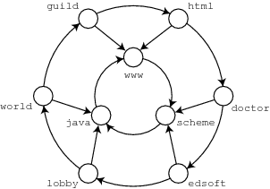
Figure 16 is a fictional web-graph fragment based very loosely on the URLs we looked at earlier. We’ll say that page p cites page q if p contains a hyperlink to q. Figure 16 is arranged in an inner and an outer ring with java, www and scheme in the inner ring and the rest in the outer ring. Java, www and scheme have three citations each, including one each from another page in the inner ring. All the other pages have one citation each. In Figure 16, java, www and scheme appear to be the authoritative pages. How might we confirm this, and indeed how might we compute some measure of their authoritativeness?
In reading papers on a given topic, scientists and scholars follow citations to learn what the papers cited add to the discussion. Usually cited papers are just skimmed — perhaps the abstract is read along with a quick look at the introduction and conclusions. However, if you keep returning to the same paper by following different chains of citations, then you might just take the time to read that paper more carefully. For the web, the analog is of a web surfer choosing at random from the hyperlinks emanating from whatever pages he is visiting. In a program, we can’t simulate a scholar skimming papers and selectively following citations, so we very roughly approximate this behavior by selecting hyperlinks at random.
| |||||||||||||||||||||||||||||||||||||||||||||||||||||||||||||||||||||||||||||||||||||||||||||||||||||
| Figure 17: Transition matrix for web-graph fragment | |||||||||||||||||||||||||||||||||||||||||||||||||||||||||||||||||||||||||||||||||||||||||||||||||||||
Figure 17 shows a table called the transition matrixfor the graph in Figure 16 in which, for example, the number in the row labeled world and the column labeled java is the probability that our surfer will jump to the java page given he is in the world page. Instead of measuring how often the surfer returns to a page — which depends on how long he surfs — we’ll measure the probability that the surfer returns to a page — which settles down (it’s said to converge) to a fixed number as the surfer continues to search the web. To show this convergence and demonstrate how to compute measures of authority, we’ll use the mathematics-savvy program Mathematica to apply some basic ideas from the theory of graphs and stochastic processes.
Mapping the row and column names in Figure 17 to the integers 1 through 9, we can represent the matrixin Figure 17 in Mathematica as (in Mathematica, semicolons distinguish separate statements or commands, much as in the C programming language; when typed at the end of a line submitted to the Mathematica interpreter, a semicolon suppresses any display of output):
In[1]:= A = {{0.0, 0.0, 0.0, 1.0, 0.0, 0.0, 0.0, 0.0, 0.0},
             {0.5, 0.0, 0.5, 0.0, 0.0, 0.0, 0.0, 0.0, 0.0},
             {0.5, 0.0, 0.0, 0.0, 0.5, 0.0, 0.0, 0.0, 0.0},
             {0.0, 0.0, 0.0, 0.0, 0.0, 0.0, 1.0, 0.0, 0.0},
             {0.0, 0.0, 0.0, 0.5, 0.0, 0.5, 0.0, 0.0, 0.0},
             {0.0, 0.0, 0.0, 0.5, 0.0, 0.0, 0.0, 0.5, 0.0},
             {1.0, 0.0, 0.0, 0.0, 0.0, 0.0, 0.0, 0.0, 0.0},
             {0.0, 0.0, 0.0, 0.0, 0.0, 0.0, 0.5, 0.0, 0.5},
             {0.0, 0.5, 0.0, 0.0, 0.0, 0.0, 0.5, 0.0, 0.0}} ;
We can represent the probable location of a surfer either initially or after surfing for a while as a vector in which the ith number is the probability of being in the ith web page. This vector is technically referred to as a probability distributionand, for rather obvious reasons, the numbers in such a vector must sum to 1. We’ll assume that initially the surfer can be in any one of the nine web pages, and so the probability distribution for the surfer’s initial location is said to be uniformand is represented as:
In[2]:= u = {1/9, 1/9, 1/9, 1/9, 1/9, 1/9, 1/9, 1/9, 1/9} ;
A vectoris represented in Mathematica as a list of numbers. In Chapter 13 we computed the dot product of two matrices, but we can also compute the dot product of a matrix and a vector. Here we define a 2 by 2 matrix and a vector of length 2 and then compute their dot product:
In[3]:= M = {{a,b},{c,d}} ;
In[4]:= v = {x,y} ;
In[5]:= M . v
Out[5]= {a x + b y, c x + d y}
The transposeof a matrix exchanges rows for columns and, again, is best understood by an example:
In[6]:= Transpose[M]
Out[6]= {{a, c}, {b, d}}
Now if we take the dot product of the transpose of the transition matrix and the vector corresponding to the surfer’s initial location:
In[7]:= Transpose[A] . u
Out[7]= {0.222222, 0.0555556, 0.0555556,
         0.222222, 0.0555556, 0.0555556,
         0.222222, 0.0555556, 0.0555556}
the ith number in this vector is the probability that the surfer ends up in the ith location after one step of randomly choosing hyperlinks, given the initial uniform distribution. To convince yourself of this, go back to the definitions of transpose and dot product and work out how the first couple of numbers in the above vector are computed; if A[i,j] is the number in the ith row and jth column of the matrix A and u[i] is the ith entry in the vector u, then, symbolically, the first number in Transpose[A] . u looks like A[java,java] * u[java] + A[lobby,java] * u[lobby] + A[world,java] * u[world] + ... + A[edsoft,java] * u[edsoft]. The resulting vector is another probability distribution.
To confirm that the result is a distribution, the following exchange exploits Mathematica’s functional programming notation: an expression of the form Apply[fun, args] applies the function fun to the arguments args and is equivalent to (apply fun args) in Scheme:
In[8]:= Apply[ Plus, Transpose[A] . u ]
Out[8]= 1
We’ve just simulated one step (or iteration) of an algorithm for determining the authoritativeness of web pages. After one step, the surfer is most likely to end up in one of the three pages, java, www or scheme, that we initially identified as the most authoritative from Figure 16. If we repeatedly execute the assignment u = Transpose[A] . u, the vector u will converge to a fixed vector called the fixed pointof the equation u == Transpose[A] . u, where == represents equality. After only 10 iterations, the probability of ending up in any web page other than java, www or scheme is quite small:
In[9]:= Do[ u = Transpose[A] . u , {10} ] ; u
Out[9]= {0.333116, 0.000108507, 0.000108507,
         0.333116, 0.000108507, 0.000108507,
         0.333116, 0.000108507, 0.000108507}
And, after 100 iterations, our random surfer is extremely unlikely to end up in any page but these three. The good news is that our algorithm lets us quickly obtain stable estimates of authoritativeness. The bad news is that none of the pages in the outer ring seem to have inherited any of the authoritativeness of the pages they link to. Indeed, it’s a fluke that the measure of authoritativeness for the pages in the inner ring is greater than that for the pages in the outer ring, however reasonable that may seem.
Some pages in the real web have no outgoing links, and so our simulated surfer would become stuck there. In our graph, all the pages have both incoming and outgoing links, but the three pages in the inner ring have no links that would let a random surfer jump outside the inner ring, and so when he eventually jumps to one of these three inner pages he will bounce around in the inner ring indefinitely.
We can fix our algorithm by modifying the transition matrix so that no matter what page the surfer is in he has some probability of ending up in any other page. Most of the time the surfer will jump more or less in accord with probabilities in the original matrix, but there is some small probability that the surfer will jump to some other page in the web graph. The fix is simple to arrange in Mathematica. First we add a small probability to every entry in the original transition matrix. The expression M + C, where M is a matrix and C is a constant, designates a new matrix whose entry in the ith row and jth column is the sum of C and the entry in the ith row and jth column of M:
In[10]:= B = A + 0.001 ;
Since each entry in the original transition matrix is meant to represent the probability of jumping from one page to another, the numbers in a given row should add up to 1. By adding 0.001 to each entry in A we’ve destroyed this property. The next computation restores the property by normalizingeach row so that its entries sum to 1. The expression Map[Function[x, body]], list] is equivalent to (map (lambda (x) body) list) in Scheme.
In[11]:= B = Map[ Function[v, v / Apply[ Plus, v ]] , B] ;
And, in another demonstration of Mathematica’s rather elegant functional programming notation, we check to make sure that the property is restored as desired:
In[12]:= Apply[ And, Table[1 == Apply[Plus, B[[i]]] , {i, Length[B]} ]]
Out[12]= True
Reinitializing the initial distribution, we run our new algorithm for a few iterations:
In[13]:= u = {1/9, 1/9, 1/9, 1/9, 1/9, 1/9, 1/9, 1/9, 1/9} ;
In[14]:= Do[ u = Transpose[B] . u , {10} ] ; u
Out[14]= {0.329209, 0.00206209, 0.00206209,
          0.329209, 0.00206209, 0.00206209,
          0.329209, 0.00206209, 0.00206209}
This turns out to be pretty close to the fixed point, as we see from a few more iterations:
In[15]:= Do[ u = Transpose[B] . u , {100} ] ; u
Out[15]= {0.329404, 0.00196464, 0.00196464,
          0.329404, 0.00196464, 0.00196464,
          0.329404, 0.00196464, 0.00196464}
In[16]:= Do[ u = Transpose[B] . u , {1000} ] ; u
Out[16]= {0.329404, 0.00196464, 0.00196464,
          0.329404, 0.00196464, 0.00196464,
          0.329404, 0.00196464, 0.00196464}
These numbers seem about right. The particular topologyof our toy web graph is a little out of the ordinary in that the inner and outer rings are rather incestuous. If we include only the links that connect from the six pages in the outer ring to the three pages in the inner ring, we’d get a set of three isolated subgraphs, each one concerned with a distinct topic. Running our algorithm, we see that the pages in the inner ring now confer significantly more of their authoritativeness on the pages that cite them:
In[17]:= Z = {{0.0, 0.0, 0.0, 0.0, 0.0, 0.0, 0.0, 0.0, 0.0},
              {1.0, 0.0, 0.0, 0.0, 0.0, 0.0, 0.0, 0.0, 0.0},
              {1.0, 0.0, 0.0, 0.0, 0.0, 0.0, 0.0, 0.0, 0.0},
              {0.0, 0.0, 0.0, 0.0, 0.0, 0.0, 0.0, 0.0, 0.0},
              {0.0, 0.0, 0.0, 1.0, 0.0, 0.0, 0.0, 0.0, 0.0},
              {0.0, 0.0, 0.0, 1.0, 0.0, 0.0, 0.0, 0.0, 0.0},
              {0.0, 0.0, 0.0, 0.0, 0.0, 0.0, 0.0, 0.0, 0.0},
              {0.0, 0.0, 0.0, 0.0, 0.0, 0.0, 1.0, 0.0, 0.0},
              {0.0, 0.0, 0.0, 0.0, 0.0, 0.0, 1.0, 0.0, 0.0}} ;
In[18]:= Z = Z + 0.001 ;
In[19]:= Z = Map[ Function[v, v / Apply[ Plus, v ]], Z ] ;
In[20]:= u = {1/9, 1/9, 1/9, 1/9, 1/9, 1/9, 1/9, 1/9, 1/9} ;
In[21]:= Do[ u = Transpose[Z] . u , {100} ] ; u
Out[21]= {0.199523, 0.0669054, 0.0669054,
          0.199523, 0.0669054, 0.0669054,
          0.199523, 0.0669054, 0.0669054}
While total isolation is rare, groups of pages do seem to form topic subgraphs that rarely cite pages outside their group. Analysis of the subgraph structure of the web is a fascinating subject that uses more of the mathematics we’ve hinted at plus fundamental results in probability and statistics.
The basic idea behind this authoritativeness measure plays an important role in the algorithms used by the Google search engine. While I don’t know exactly how Google works, a good guess is that it uses traditional sorts of information retrieval to obtain an initial set of pages, then ranks these pages using some combination of authoritativeness and various measures of document similarity such as the term-frequency methods we discussed. With this hint, it’s interesting to submit queries to Google and then do various experiments analyzing the content and the links for the pages returned.
Link-based measures of authority are open to various schemes for artificially improving the authoritativeness of pages. For example, I could create pages with lots of links to my own pages (tantamount to citing your own work), pay lots of people to put links to my pages on their pages, or conspire with a bunch of other folks to cite one another. None of these tricks work particularly well on Google, but other, more complicated schemes that exploit both document similarity and link-based measures of authority require the folks at Google and every other search-engine company continually to improve their algorithms. To learn more about information retrieval techniques for searching the web, check out Soumen Chakrabarti’s Mining the Web: Discovering Knowledge from Hypertext Data.
14.4 Searching for exotic fruit
Most search engines let you search for nontext sources of information such as images, music and movies. Such nontext sources present a whole new set of challenges for search algorithms. In an ideal world, images would be stored as structured data in relational databases. Databases store all sorts of information besides text and numbers, and we could use a variant of the music database in Chapter 3 to store textual information about songs and albums as well as the music itself, encoded in a digital format such as MP3.5 Unfortunately, image and music data on the wild web is not so conveniently stored and catalogued.
Most current techniques for searching the web for nontext-based information rely on using “nearby” text to index the nontext data. Image data is typically included in web pages using the IMG HTML tag, and so a statement such as <IMG src="images/adirondack.gif"> embedded in a web page would cause the specified image in “graphics interchange format” to be downloaded and then displayed in a browser window. If you’re really lucky, the person who created the web page may have used the ALT attribute for IMG to give a textual description of the image, for example, <IMG src="images/adirondack.gif" ALT="adirondack chair">. The ALT attribute is useful as an alternative method of display in text-only browsers like lynx or even in a graphical browser if you’re on a slow connection or have turned off graphics downloading for some other reason.
Hyperlinks in HTML are specified using the A (for “anchor”) tag, and the “clickable” text that’s displayed in your browser, usually underlined, emboldened or otherwise highlighted, is called the anchor text. For example, a web page for an online store featuring outdoor patio and garden furniture might contain this line of HTML code:
<A HREF="http://www.outdoors.com/adirondack.htm">adirondack chair</A>
When viewed with a browser, the anchor text adirondack chair is highlighted; if you click on this text, you’ll jump to the indicated web page, which might feature images of chairs. You can also use images instead of text to anchor hyperlinks, in which case the pages they point to may yield clues about the image content. The online furniture store might display small product images called thumbnailsthat link to descriptions of the product, as in
<A HREF="adirondack.htm"><IMG SRC="images/adirondack.gif"></A>
Now when you click on the thumbnail image adirondack.gif you jump to the description of the chair, which may include more images.6 There are all sorts of tricks for finding text that is associated with images and can be used for indexing; if suitable text can be found, then the problem of searching for images reduces to searching for text.
There are also efforts afoot to use so-called image understanding and pattern recognition methods from the field of machine vision to extract clues directly from image data, but current techniques along these lines are at the bleeding edge of technology and not yet ready for prime time. In addition to searching still images, researchers are developing techniques for searching video images. Imagine a reporter for a cable news service wanting to search the studio’s video archives for footage of Keanu Reeves getting out of a limousine for a news segment she’s doing. A program to do this would have to identify the actor, distinguish a limousine from other objects, and somehow recognize a segment in which someone exits from a limo.
Whether extending traditional information-retrieval methods for searching text documents or developing new methods to search multimedia data, there’s a lot of very interesting work to be done. Relevant techniques can be found in the study of linguistics, natural-language processing, speech recognition, image processing, machine vision and artificial intelligence. And, as fast as researchers figure out how to make sense of existing formats and media, artists and technologists will come up with new and richer ways of expressing themselves that will require even more sophisticated search methods.
1 Remember that the web can be thought of as a huge graph, a directed graph with cycles and billions of nodes. You can search such a graph using depth-first or breadth-first search, but you do have to be wary of cycles, otherwise you’ll waste a lot of time repeatedly visiting the same nodes.
2 I couldn’t find a generally available Unix command to produce a word histogram for a file, but in the spirit of Perl’s “There’s more than one way to do it”, here’s a shell script that does the trick and more or less fits on a single line: cat file.txt | tr -dc "a-zA-Z’ \n" | tr " " "\n" | sort | uniq -c | sort -k1,1nr -k2. Its main drawback, a common problem with short programs, is that it takes much longer to explain than to write down. You may recall the trick of using sortfollowed by uniq from Chapter 12. It’s a useful exercise to figure out how this script works and then experiment with variations on the basic theme. Here’s how the pieces play together: tr translates characters; the first invocation, tr -dc "a-zA-Z’ \n", deletes (the d in -dc) the complement (the c in -dc) of the characters specified in its first and only argument (all alphabetic characters plus the apostrophe, space and new-line characters (\n) characters), and the second invocation, tr " " "\n" , translates all spaces to new-line characters, thereby ensuring that each line contains at most one word. sort sorts lines; its first invocation makes sure that lines containing the same word appear consecutively in the output, thus paving the way for uniq, which filters out consecutive identical lines in a file; the -c option directs uniq to precede each line with the number of times the line appears in the input. The final invocation of sort uses some tricky directives to sort the output of uniq so that the most frequently occurring words appear first and those occurring the same number of times appear alphabetically.
3 Most information-retrieval systems preprocess the data much more extensively than I have. In addition to converting all the text to lower-case letters and eliminating punctuation, most systems remove common stop words like “a”, “an” and “to” that add little information to a document summary. Many systems also use various stemmingalgorithms to map words to a common root — for example, the words “sink”, “sinks” and “sinking” would all be mapped to “sink.” Stemming conflates words, which sometimes you want and sometimes causes confusion: for example, “universe”, “universal” and “university” are all mapped to the root “univers”. Sophisticated stemmers use a combination of morphological analysis — remove all “ing” endings — and lexical analysis — check to see if the words mapped to the same root have similar meanings. Not surprisingly, the methods used to preprocess a list of words prior to analysis can make a huge difference in performance.
4 The location of a point in three-dimensional (Euclidean) space is specified by its x, y and z coordinates. The Euclidean distance between two points (x1,y1,z1) and (x2,y2,z2) is the length of the path connecting them and is calculated as the square root of the sum of the squares of the differences of their respective coordinates √((x1 - x2)2 + (y1 - y2)2 + (z1 - z2)2).
5 MP3 is the compression format used in a popular method of encoding digital audio files. The analog audio signal produced in recording an album is digitized by reading off and then storing values (“samples”) of the signal at discrete time points (44,100 samples per second for audio CDs). The sampled data is stored as a sequence of integers in a file. To reduce the amount of storage required and speed downloading, this file is compressed by converting the data to a more compact format. A compression format might allow a compression algorithm to convert a sequence like 1742, 1742, 1742, 1742, 1742 into a specification like 1742 (5) or, in “lossy” compression, a sequence like 3241, 3242, 3241, 3241, 3239 3241 into the specification 3241 (6) which only approximately captures the original uncompressed data. The acronym MP3 derives from another acronym, MPEG (“motion picture experts group”), referring to a set of layered formats for compressing audio and video, and one format in particular, “Layer 3”, which is the basis for MP3.
6 The two examples using the HTML anchor tag demonstrate the two modes of specifying URLs allowed by the HTTP protocol, relative and absolute path names, which directly correspond to the two methods of specifying files and directories in most modern file systems.