Chapter 13

Forest for the Trees

Often when you’re trying to solve a problem, you pull out a pen or pencil and grab a handy piece of paper to write down a column of numbers, draw a diagram, or make a list. In solving the problem, you might sum the numbers, trace lines in the diagram, or match items of the list with items of a second list. These auxiliary scribblings are used to organize information — as with the list or column of numbers — or represent objects so they can be easily manipulated — as with the diagram. Data structuresare the algorithmic analog of these handy pieces of paper.

In Chapter 11 we saw that browsers and web servers in a computer network exchange information by bouncing small packages of data from one computer to another until they arrive at their final destination. How can we represent a computer network so that an algorithm can figure out what sequence of computers to use in transferring a data package? For that matter, how do we represent airline schedules, circuit diagrams, computer file systems, road maps and medical records so that they can be manipulated algorithmically?

Many algorithms use special data structures to represent their inputs and outputs or to perform intermediate calculations. In Chapter 7 we used lists and vectors to keep track of journal entries. In Chapter 10 we learned how to use a stack to keep track of the contents of registers in nested subroutine calls. We’ve also seen even more basic data structures: strings and integers are among the simplest of “primitive data types”. Other primitive data types include characters, other varieties of numbers (single and double floating-point numbers, rationals, short integers and long integers), and pointers that let you directly address locations in memory.

But when computer people talk about data structures, they’re usually referring to compositedata types that let you organize multiple instances of the same data type or combine instances of several primitive (or composite) data types. All the obvious organizing strategies are generally available, including bags(which assume no particular order), lists (which assume a linear ordering and are often called arrays), and tables (in which items are arranged vertically and horizontally in a grid and which are often called two-dimensional matrices). There are also more specialized composites like association lists(which, like telephone books, store information, like telephone numbers, under various keys, like individuals’ names) and the records and relational tables that we saw in Chapter 3.

But no discussion of data structures is complete without some mention of graphsand their various important subclasses, including directed graphs, directed acyclic graphs and, perhaps the most important and useful class of graphs of all, trees. Graphs are everywhere in computer science; indeed, while we didn’t make a fuss over them, you’ve already seen several examples of graphs in earlier chapters.

13.1  Graph theory

Graph theory is a subarea of discrete mathematics (that’s the part of mathematics that deals with discrete, separable and often countable objects rather than, say, the continuous variables of calculus and real analysis) that is particularly relevant to computer science. The mathematics can be pretty abstract but the applications are everywhere and very concrete. A computer network, a web site, the entire World Wide Web, and a hierarchical file system containing directories and files can all be thought of as graphs.

Mathematically, a graph is a set of nodes(also called vertices) and a set of links(also called edges). A link is specified by a pair of nodes and can be either one-way (unidirectional) or two-way (bidirectional). The distinction between one-way and two-way links can be used to model the difference between connections that allow information to flow in both directions or in only one direction. Graphs are usually drawn by depicting the nodes as circles and the links as lines (bidirectional) or arrows (unidirectional). Sometimes the nodes are labeled, as in these three examples:

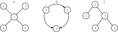Graph theorists and computer scientists like to talk about the topologyof a graph: A is a graph with a star topology, B (ignoring the arrows) has a ring topology and C has a tree topology.

Think about how we might represent a network of computers as a graph. Simplifying somewhat, computers are connected via cables to various pieces of equipment including other computers and specialized connection boxes variously called switches, hubs, routers and bridges (you’d need a short course in computer networks — or a browser, a search engine and patience — to understand the differences among these). Some of the “cables” can be a little complicated — for example, a serial cable from a computer to a modem that via a phone line communicates with a second modem connected by another serial cable to a second computer. But the basic idea is that there is some way of sending information back and forth along the cable between the devices attached to either end.

Computers in the same building are often connected via hubs and switches to form a local-area network (LAN). LANs are typically organized in graphs with star or ring topologies. Large computer networks are configured (hierarchically) at multiple levels so that whole chunks of the network at one level correspond to the simplest atomic components at the next higher level. Computers within a company can be arranged as a wide-area network (WAN) containing one or more LANs. In some cases, it makes sense to think of a WAN as a graph whose nodes consist of LANs. Then there are metropolitan-area networks (MANs) and global-area networks, some of whose connections might be via satellite or cables laid along ocean beds. The graphs corresponding to these larger, continent-spanning networks can be thought of as having WANs and MANs for nodes.

Generally, all the links in a particular graph are either one-way or two-way, and we refer to a graph with all one-way links as directedand a graph with all two-way links as undirected. It usually makes sense to represent computer networks as undirected graphs since communication is bidirectional. Assuming that only one link connects any two nodes, we can unambiguously specify any link as an ordered pair of nodes in which the “arrow” points from the first node in the pair to the second in the case of directed graphs or as an unordered (the order doesn’t matter) pair in the case of undirected graphs. Example A is an undirected graph that we can represent as a set of five nodes {1,2,3,4,5} and a set of four links {{1,2},{1,3},{1,4},{1,5}}. Similarly, we can represent the directed graph B as a set of three nodes {1,2,3} and a set of three (directed) links {{1,2},{2,3},{1,3}}.

Graph theory is full of terms and definitions that turn out to be useful in describing physical systems; I’ll give you a little taste. A pathfrom one node to a second node in a graph is a sequence of nodes and links of the form node₁ (read “node sub one”), link₁, node₂, link₂, ..., link_n-1, node_n, where node₁ is the beginning of the path and node_n is the end of the path. In graph A, there is an undirected path from the node labeled 2 to the node labeled 4 defined by {2,{1,2},1,{1,4},4}. In graph B, there is a directed path from the node labeled 1 to the node labeled 3 defined by {1,{1,2},2,{2,3},3}. There is also an undirected path from 4 to 2 in A defined by {4,{1,4},1,{1,2},2}, but there is not a directed path from 3 to 1 in graph B. We might imagine an undirected version of B, call it B’, in which all the one-way links are replaced by two-way links, so that there is an undirected path in B’ from 3 to 1.

A graph is said to be connectedif there is a path between all pairs of nodes in the undirected version of the graph. A circuit is an undirected path that begins and ends at the same node and has at least one link.¹ A tree is an undirected graph that is both connected and circuit free. A and C are trees but B’ is not because it contains a circuit {1,{1,2},2,{2,3},3{1,3},1}.

A cycle in a directed graph is a directed path that begins and ends at the same node and has at least one link. A directed graph that doesn’t contain any cycles is called a directed acyclic graph or DAG; B is a DAG.

There’s also a directed version of trees. A directed graph is said to have a rootnode r if there is directed path from r to every other node in the graph. The node labeled 1 is a root of B. A directed graph is called a directed tree if it has at least one root and its underlying undirected graph is a tree. B is not a directed tree, but imagine a directed version of C, call it C’, with all its links pointing down (toward the bottom of the page). C’ is a directed tree and the node labeled 1 is its only root.

In a directed graph, the parents of a node are all those nodes that have links pointing to the node, and the children of a node are all those nodes that have links pointed to starting from that node. A node can have 0, 1, 2 or more parents and any number of children, including none at all. In C’, node 1 has no parents and two children, 2 and 3, while node 5 has one parent, 3, and no children.

A subgraphis part of a graph. The graph consisting of nodes {3,4,5} and links {{3,4},{3,5}} is a subgraph of C; indeed, it’s a subtreeof C.

Mathematicians like graph theory because both the mathematics and the graphs themselves are beautiful. Computer scientists like graph theory for the same reasons and also because they can use it to analyze algorithms that operate on graphs, or things like computer networks that can be represented as graphs. For example, there’s an algorithm due to Edsger Dijkstrathat finds the shortest path between any two nodes in a graph using a number of primitive operations that scales polynomially in the number of nodes and links in the graph. This result is important because it tells us that packages of data in computer networks can be routed relatively efficiently.

So how would you actually go about representing a graph in a form (data structure) that a computer could use? We can use the mathematical notation introduced earlier almost directly. Indeed, Mathematica would be quite happy representing graph B as a pair

{{1,2,3},{{1,2},{1,3},{2,3}}}, 

in which the first element of the pair is the list of nodes and the second element is the list of links. And Lisp (or Scheme) would have no trouble using its list notation to represent graph B, with the curly brackets replaced by parentheses (what else!) and commas replaced by spaces:

((1 2 3) ((1 2) (1 3) (2 3)))

Another convenient representation is as a list of pairs, one for each node, in which the first element of each pair is the node (or the label for the node) and the second element is a list of nodes (possibly empty) the node is linked to. This is called the adjacency-listrepresentation since it includes a list of the nodes that are adjacent to each node in the graph. Here is graph B in Mathematica using this representation:

{{{1,{2,3}},{2,{3}},{3,{}}}}

or in Lisp:

((1 (2 3)) (2 (3)) (3 ()))

In an adjacency list, we no longer need keep around a separate list of all the nodes, since each node is represented as a pair consisting of the label of the node along with a list of the labels of all of its adjacent nodes.

13.2  Graph algorithms

Now that we can encode graphs in a programming language, let’s see what we can do with them. Graph algorithms, that is, algorithms that operate on graphs, are a particularly important subarea of algorithms. Their applications include routing delivery vehicles, designing cellular networks and laying out digital circuits, as well as a host of problems involving computer and communication networks.

It’s often useful to determine whether or not there is a path from one node in a graph to another, and algorithms that find such paths are called graph-searching algorithms. Let’s take a look at a Scheme version of one the most basic (and important) such algorithms; it’s called dfs_path? because it tells you whether or not a path exists using depth-first search(DFS), a strategy for searching graphs that we’ll explain shortly.

(define (dfs_path? graph queue goal max_steps)
  (if (or (empty_queue? queue)
          (= max_steps 0))
      "no"
      (if (= (first_node queue) goal) 
          "yes"
          (dfs_path? graph 
                     (append (get_links (first_node queue) 
                                        graph)
                             (remaining_nodes queue))
                     goal
                     (- max_steps 1)))))

We’ll also need some auxiliary functions whose definitions (with one exception) I hope you won’t worry about too much, since they’re not critical for understanding how depth-first search works. Just interpret the function names as you would English; for example, (first_node queue) means return the first (car) node off the queue, (remaining_nodes queue) means return the rest (cdr) of the nodes on the queue (minus the first), (empty_queue? queue) returns the Scheme equivalent of true if the queue is empty and false otherwise, and (initialize_queue node) returns a list consisting of a single item, node.

(define (first_node queue) (car queue))
(define (remaining_nodes queue) (cdr queue))
(define (empty_queue? queue) (null? queue))
(define (initialize_queue node) (list node))

The function get_links is a little more complicated:

(define (get_links node graph) (cadr (assoc node graph)))

The get_links function uses the association-listdata structure, which is often useful in designing algorithms.² Here’s how assoc, a Scheme function for extracting information from association lists, is used to extract the list of links associated with a node in a graph represented in adjacency-list format:

> (define G '((1 (2 3)) (2 (3 4)) (3 ()) (4 ())))
> (assoc 2 G)
(2 (3 4))

The single quote “’” in the define statement tells Scheme to treat as literal the expression immediately following (delimited by the opposite balancing parenthesis), and, in particular, not to treat it as an attempt to call a function. The function cadrreturns the second element in a list ((cadr ’(1 2 3)) returns 2), and so (get_links 2 G) returns the list (3 4).

Back to depth-first search. Here’s a paraphrase of what the function dfs_path? does. The function is called with four arguments: a graph in adjacency-list format, a queue of nodes to explore next (which initially contains only the starting node), a destination (or goal) node, and an integer indicating the maximum number of steps to take before calling it quits; dfs_path? returns "yes" if it finds a path from the starting node to the goal and "no" if it doesn’t.

If the queue is empty or you’ve used up your allowance of steps, then you’re done and dfs_path? returns "no". Otherwise, if the first node on the queue is the goal node, then you’re also done and it returns "yes". If neither of these conditions holds, then max_steps must be greater than zero and there’s at least one more item on the queue. So in this case call dfs_path? recursively with the same graph, a new queue that we’ll describe presently, the same goal, and max_steps less one. The new queue contains all the nodes reachable by following a link starting at the first node on the queue appended³ to the list of all nodes remaining on the queue minus the first (since we’ve now determined it isn’t the goal).

Now let’s see if it works. First, we use the single-quote mechanism to load the adjacency-list representations for the example graphs A, B and C:

(define A '((1 (2 3 4 5)) (2 (1)) (3 (1)) (4 (1)) (5 (1))))
(define B '((1 (2 3)) (2 (3)) (3 ())))
(define C '((1 (2 3)) (2 (1)) (3 (1 4 5)) (4 (3)) (5 (3))))

Is there a path from 1 to 3 in graph B? Let’s give dfs_path? a maximum of 10 steps to find an answer, where each step corresponds to traversing a link in the graph:

> (dfs_path? B (initialize_queue 1) 3 10)
"yes"

Sure enough. What about from 3 to 1?

> (dfs_path? B (initialize_queue 3) 1 10)
"no"

Right again. What about from 1 to 5 in graph C?

> (dfs_path? C (initialize_queue 5) 1 10)
"yes"

We’re on a roll. DFS is mighty useful and you’ll find it cropping up as a subroutine in all sorts of algorithms. But DFS has some drawbacks and it isn’t the method of choice for searching all graphs. Time to draw another bunch of graphs:

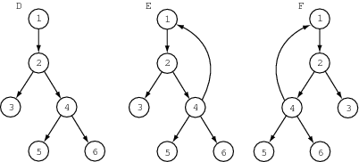Graph D is a tree and would be described as a list of nodes and links as

{{1,2,3,4,5,6},{{1,2},{2,3},{2,4},{4,5},{4,6}}}

and in adjacency-list format as

{{1,{2}},{2,{3,4}},{3,{}},{4,{5,6},{5,{}},{6,{}}}}.

E is just like D except that a cycle was introduced by adding a link from 4 to 1:

{{1,2,3,4,5,6},{{1,2},{2,3},{2,4},{4,1},{4,5},{4,6}}}

It’s a pretty common sort of graph, though not a tree nor a DAG (directed acyclic graph). In adjacency-list format, it looks like

{{1,{2}},{2,{3,4}},{3,{}},{4,{1,5,6},{5,{}},{6,{}}}}

Finally, F is really the same as E: it’s the mirror image of E. Here’s the adjacency-list format:

{{1,{2}},{2,{4,3}},{3,{}},{4,{1,5,6},{5,{}},{6,{}}}}

I’ve thus reversed the order in which 3 and 4 appear in the lists of nodes adjacent to 2; as we’ll see, this turns out to make a crucial difference to DFS. We define these graphs in Scheme as:

(define D '((1 (2)) (2 (3 4)) (3 ()) (4 (5 6)) (5 ()) (6 ())))
(define E '((1 (2)) (2 (3 4)) (3 ()) (4 (1 5 6)) (5 ()) (6 ())))
(define F '((1 (2)) (2 (4 3)) (3 ()) (4 (1 5 6)) (5 ()) (6 ())))

Let’s see if there is a path from 1 to 4 in D:

> (dfs_path? D (initialize_queue 1) 4 10)
"yes"

Yep. How about in E?

> (dfs_path? E (initialize_queue 1) 5 10)
"no"

That can’t be right! E has all of D’s links plus one. If there’s a path from 1 to 5 in D there has to be a path in E.

We can modify dfs_path? just slightly so that it detects the path in E. The following function, called bfs_path? for breadth-first search(BFS), is defined just as dfs_path? with the exception of the order of the arguments in the call to append. This small change makes BFS explore the graph by traversing links in the order in which they are loaded onto the front of the queue. BFS looks at all nodes reached by paths of length n before it looks at any of the nodes that can be reached only by a path of length greater than n. DFS searches by plunging deeper and deeper into the graph — hence the name depth-first search.

(define (bfs_path? graph queue goal max_steps)
  (if (or (empty_queue? queue)
          (= max_steps 0))
      "no"
      (if (= (first_node queue) goal) 
          "yes"
          (bfs_path? graph 
                     (append (remaining_nodes queue)
                             (get_links (first_node queue) 
                                        graph))
                     goal
                     (- max_steps 1)))))

With bfs_path? we get the answer we expected earlier:

> (bfs_path? E (initialize_queue 1) 5 10)
"yes"

Neither dfs_path? nor bfs_path? can tell when they’ve previously visited a node in the graph, and so, starting from node 1, both algorithms may return to 1, having followed the path {1,{1,2},2,{2,4},{4,1},1} and then again having followed {1,{1,2},2,{2,4},{4,1},1,{1,2},2,{2,4},{4,1},1}, and so ad nauseam. We could fix this by having both algorithms remember where they’ve been.

If we were to remove the link from 4 to 1 in F and ask to check for a path from 1 to 6, DFS would traverse the graph in depth-first order, 1, 2, 4, 5, 6, 3, and BFS would traverse the graph in breadth-first order, 1, 2, 4, 3, 5, 6. Try to think of cases in which DFS is the better choice (hint: consider graphs without cycles in which the goal is some considerable distance from the starting node) and cases in which BFS is the better choice (hint: consider very large graphs in which the goal is not far from the starting node and each node has few children). Graphs are easy to sketch on paper and such sketches help a lot in testing your intuitions.

Often, in addition to knowing whether or not a path exists, you’d like to see the path, perhaps multiple paths if there are several. We could modify dfs_path? and bfs_path? to return paths, but instead I’m going to show you an alternative way to write a search algorithm that illustrates another model of computation touched on in Chapter 1.

In dfs_path? and bfs_path?, the recursive call picks out one node to follow from the queue, and passes on the rest of the nodes as an argument to the recursive call. Suppose we could generate a separate recursive call for each possible new link to follow; then we could generate a recursive call with a new starting node and include the path information as an additional argument. We wouldn’t even need to keep a queue around, since we’d immediately spin off a recursive call for each possible link out of the current node.

Scheme provides a nice way of spinning off such recursive calls or, more generally, applying a procedure multiple times to different sets of arguments. It involves what are called mapping operators and is part of a more general approach to programming called functional programming. Mapping operators have appeared in many different programming languages over the years and once you start using them it’s hard to stop.

The special operator maptakes a procedure that has some number of formal parameters n and a set of n lists each of length m for some arbitrary m. You can think of map as applying the procedure not to each list of arguments but to what’s called a cross sectionof all the lists. The first cross section consists of the first item in the first list, the first item of the second list, and so on. The procedure is applied to this first cross section and then to the second cross section consisting of the second item in the first list, the second item in the second list, ..., and so on until the procedure has been applied to all m cross sections. In the expression (map + ’(1 2 3) ’(1 2 3)), the procedure + is applied to (+ 1 1), (+ 2 2), and (+ 3 3), and the results are returned as a list:

> (map + '(1 2 3) '(1 2 3)) 
(2 4 6)

The map operator accepts any procedure including the kind with no name that we can specify using lambda, as we saw in Chapter 6:

> (map (lambda (x y z) (- (* x y) z)) 
       '(2 3)
       '(3 4)
       '(1 2))
(5 10)

Here’s the definition of our procedure to search for and report as many paths as possible. We can no longer count all the steps taken in all the recursive calls, but we can do something that in many cases is even better: we can put a limit on how deep (the number of links traversed) we want any recursive call to search. This procedure explores the graph in breadth-first search and so inherits both the advantages and disadvantages of that method.

(define (find_all_paths graph begin end path max_depth)
  (if (= begin end) 
      (display_path (extend_path end path))
      (if (> max_depth 0)
          (map (lambda (new_begin)
                 (find_all_paths graph
                                 new_begin 
                                 end  
                                 (extend_path begin path)
                                 (- max_depth 1)))
               (get_links begin graph))))
  "done")

In order to understand how find_all_paths works, we also need some auxiliary functions that hide details you don’t need to know:

(define (display_path path) (printf "Path: ~A~N" (reverse path)))
(define (initialize_path) (list))
(define (extend_path node path) (cons node path))

Let’s give it a whirl on graph B:

> (find_all_paths B 1 3 (initialize_path) 10)
Path: (1 2 3)
Path: (1 3)
"done"

It doesn’t do any better than dfs_path? or bfs_path? on graphs with cycles; in fact, it can be downright distracting:

> (find_all_paths E 1 3 (initialize_path) 24)
Path: (1 2 3)
Path: (1 2 4 1 2 3)
Path: (1 2 4 1 2 4 1 2 3)
Path: (1 2 4 1 2 4 1 2 4 1 2 3)
Path: (1 2 4 1 2 4 1 2 4 1 2 4 1 2 3)
Path: (1 2 4 1 2 4 1 2 4 1 2 4 1 2 4 1 2 3)
Path: (1 2 4 1 2 4 1 2 4 1 2 4 1 2 4 1 2 4 1 2 3)
Path: (1 2 4 1 2 4 1 2 4 1 2 4 1 2 4 1 2 4 1 2 4 1 2 3)
"done"

But again we could fix this by keeping an extra argument to remember all the places we’ve visited before.

When I started writing about the adjacency-list format, I resolved to say something about another handy representation for graphs called adjacency matrices. But before we can represent an adjacency matrix, it might be a good idea to learn how to represent a regular old matrix. An n by m matrix⁴ is a table consisting of (n * m) numbers arranged in n rows and m columns; typically we represent such a matrix as n lists each of length m, so that a 2 by 3 matrix all of whose entries are 1 would look like {{1,1,1},{1,1,1}}.

To represent a graph with n nodes as an adjacency matrix, you associate the nodes in the graph with the integers 1 through n and construct an n by n matrix such that the entry in the jth column of the ith row is 1 if there is a directed link in the graph from the ith node to the jth node and is 0 otherwise. Using the labels of the nodes of graph B {{1,2,3},{{1,2},{1,3},{2,3}}} as the associated integers, the adjacency matrix for B would be

{{0,1,1},
 {0,0,1},
 {0,0,0}}

Adjacency matrices are useful for representing small graphs and larger graphs that have lots of links. A graph with n nodes can have as many as n² links (since any pair of nodes could have two directional links linking them together), and an adjacency matrix for a graph with n nodes has exactly n² entries.

Mathematica likes graphs represented as adjacency matrices, just the way I entered the matrix for B. Mathematica even has nifty functions for displaying matrices so they are easy to decipher:

In[1]:= TableForm[ {{0,1,1},{0,0,1},{0,0,0}} ]

Out[1]= TableForm= 0   1   1

                   0   0   1

                   0   0   0

Mathematica also has very convenient operators for combining matrices and vectors(one-dimensional matrices) that are very useful in linear algebra, another branch of mathematics important in computer science, especially in graphics and robotics. I can use Mathematica’s facility with symbolic operations to show you what it means to add two 2 by 2 matrices together:

In[2]:= TableForm[ {{a,b},{c,d}} + {{e,f},{g,h}} ]

Out[2]= TableForm= a + e   b + f

                   c + g   d + h

and to take their inner product(also called the dot product):

In[3]:= TableForm[ {{a,b},{c,d}} . {{e,f},{g,h}} ]

Out[3]= TableForm= a e + b g   a f + b h

                   c e + d g   c f + d h

You’ll need a larger example to generalize, so I’ll throw in the dot product of two 3 by 3 matrices:

In[4]:= TableForm[ {{a,b,c},{d,e,f},{g,h,i}} . 
                   {{j,k,l},{m,n,o},{p,q,r}} ]

Out[4]= TableForm= 
           a j + b m + c p   a k + b n + c q   a l + b o + c r

           d j + e m + f p   d k + e n + f q   d l + e o + f r

           g j + h m + i p   g k + h n + i q   g l + h o + i r

If we take the dot product of an adjacency matrix with itself,

In[5]:= TableForm[ {{a,b},{c,d}} . {{a,b},{c,d}} ] 

Out[5]= TableForm=  a a + b c   a b + b d

                    a c + c d   b c + d d

the entry in the jth column and ith row of the resulting matrix tells us if it’s possible to get from i to j by traversing a path consisting of exactly one link. In general, if Mⁿ is the matrix we obtain by taking the dot product of an adjacency matrix with itself n times (for example, M³ = M.M.M), then the entry in its jth column and ith row tells us if it’s possible to get from node i to node j by traversing a path consisting of exactly n links. If you add together all of the matrices M¹, M², ..., Mⁿ you get a matrix in which the entry in the jth column and ith row tells us how many different paths connect node i to node j by traversing n or fewer links.

Here’s the adjacency matrix for graph F:

In[6]:= F = {{0,1,0,0,0,0},
             {0,0,1,1,0,0},
             {0,0,0,0,0,0},
             {1,0,0,0,1,1},
             {0,0,0,0,0,0},
             {0,0,0,0,0,0}}

Here’s the same matrix displayed in a somewhat easier-to-read format:

In[7]:= TableForm[ F ]

Out[7]= TableForm= 0   1   0   0   0   0

                   0   0   1   1   0   0

                   0   0   0   0   0   0

                   1   0   0   0   1   1

                   0   0   0   0   0   0

                   0   0   0   0   0   0

And now we compute a new matrix in which the entry in the jth column and ith row indicates how many different paths of length four or less connect node i to node j:

In[8]:= TableForm[ F . F + 
                   F . F . F + 
                   F . F . F . F + 
                   F . F . F . F . F ]

Out[8]= TableForm= 1   1   2   2   1   1

                   2   1   1   1   2   2

                   0   0   0   0   0   0

                   1   2   1   1   1   1

                   0   0   0   0   0   0

                   0   0   0   0   0   0

We’re actually searching this graph by performing matrix operations; the resulting matrix tells us whether there is a path connecting any pair of nodes and if so how many. This isn’t the method of choice for most graph-searching problems, but a variant of it will turn out to be useful when we consider searching the World Wide Web in Chapter 14. First, let’s consider some other applications that involve graphs.

13.3  File systems as graphs

The directories in most file systems in most operating systems are arranged as trees. Using a command-line-oriented interface such as a shell or, more typically nowadays, some sort of a graphical interface, you can create (make) new directories using mkdir, remove an existing directory with rmdir, change your current working directoryusing chdiror list the contents of a directory using ls.

I have an alias (think of it as a little program) called cd⁵ that I use instead of chdir and that, in addition to allowing me to change my current working directory, changes my prompt to help me keep track of where I am in the file system (it’s really easy to get lost). This program first initializes the prompt shell variable, which determines what the shell prints at the beginning of a line. It then defines (alias is a little like define in Scheme) cd as a program that first calls chdir and then resets the prompt by referring to the cwd shell variable that the system uses to keep track of my current working directory:

set prompt = "$cwd % " 
alias cd 'chdir \!* ; set prompt = "$cwd % "'

The expression \!* appearing in an alias refers to the arguments of the command being defined, cd in this case, when the command is read by the shell; thus, for example, my typing cd /u/tld/ is transformed into chdir /u/tld/ ; set prompt = "$cwd % ". This little program resides in a file (named .cshrc in my top-level directory) with a lot of other useful little programs that are evaluated every time I start up a shell. I use it many times a day and hardly ever thought about it until in working on this chapter I wondered how it would handle graphs with cycles — yes, you can create cycles in file systems.

I’m going to invoke mkdir and create a tree just like graph D in the previous section:

/u/tld % mkdir one 
/u/tld % cd one 
/u/tld/one % mkdir two 
/u/tld/one % cd two 
/u/tld/one/two % mkdir three four 
/u/tld/one/two % cd four 
/u/tld/one/two/four % mkdir five six 
/u/tld/one/two/four % ls 
five  six 
/u/tld/one/two/four % cd ..
/u/tld/one/two/ % ls
four three
/u/tld/one/two/ % cd four
/u/tld/one/two/four % ls 
five  six 

In the shell “..” always means the parent directory of the directory you’re currently in. With the exception of symbolic links (which we’ll get to in a moment), each directory has a unique parent directory.

Each time I invoked cd it correctly redisplayed the prompt showing my location in the directory structure. Now I’m going to create a symbolic linkusing the link command lnwith the symbolic (-s) option.⁶ The link command takes as arguments the path to the destination directory (the destination of the link) and a name for the link (considered to symbolically represent the destination). We’ll set the name to be the same as the name of the destination directory:

/u/tld/one/two/four % ln -s /u/tld/one one 
/u/tld/one/two/four % ls 
five  one   six 

Now we have a graph with a cycle in it that is exactly the same as graph E above (and graph F, since E and F are really just different drawings of the same graph). But now watch what happens as we walk around on the graph traversing links:

/u/tld/one/two/four % cd one 
/u/tld/one/two/four/one % cd two 
/u/tld/one/two/four/one/two % cd four 
/u/tld/one/two/four/one/two/four % cd one 
/u/tld/one/two/four/one/two/four/one % cd two 
/u/tld/one/two/four/one/two/four/one/two % cd four
/u/tld/one/two/four/one/two/four/one/two/four/ %

Just as find_all_paths was fooled by cycles in graph E, so my little cd program has become confused, thereby confusing me as well with its prompt that encodes my entire cyclic traversal. Luckily, another program called pwd provides a more reasonable and cycle-free report of my working directory as the shortest path from the root, “/”, to my working directory. It turns out that “u” was another symbolic link that I’d completely forgotten about.

/u/tld/one/two/four/one/two/four/one/two/four/ % pwd
/home/tld/one/two/four

The fact that you can create trees and graphs using directories means that you can create data structures for storing your stuff right on top of your computer’s file system. For example, in Chapter 1 I described a tree-like structure of files and directories that I used to organize my journal entries. I expect you can think of similar ways to keep track of old email messages, digital photos or music files.

13.4  The web graph

This notion of file systems (and hence graphs) as efficient ways of organizing information is pretty useful, and before we leave the subject, I’d like to say a few words about the mother of all file systems, the World Wide Web. The World Wide Web, perhaps the largest artifact ever, can be modeled quite naturally as a graph with the web pages as nodes and the hyperlinks as links. We talked at length in Chapter 11 about the technology that makes the World Wide Web possible and we’ll visit the web again in Chapter 14, but for now I just want you to think about it as a graph.

The web graph, as it is now called, has billions of nodes. That’s such a big graph that in searching for information in it, you might as well think of it as infinitely large.⁷ Assessing the size of the web is complicated by the fact that lots of it is virtual — many of its pages, such as those showing merchandise at online stores, don’t exist until someone wants to see them; they’re created on the fly and often personalized in content and format for a particular customer.

Strictly speaking, the web graph is a directed graph with cycles; hyperlinks tell you how to go from the page you’re on to the page they point to, but you have to do more work — search the graph exhaustively or nearly so — in order to find out what other pages point to a given page. However, we can uncover interesting structure in the web graph just by looking at how web pages are connected to one another, without even looking at their contents. We’ll need a couple of technical terms and definitions to talk about this structure more precisely.

A strongly connected graphis a directed graph that has a directed path from each node to every other node. A strongly connected component, C, is a strongly connected subgraph of a directed graph, G, such that no node in G can be added to C and it still be strongly connected. A sinkin a graph is a set of nodes that have no links to nodes outside the set. The web graph has sinks corresponding to connected components that have incoming hyperlinks but no outgoing links: once you enter a sink, you can’t exit simply by following hyperlinks. It also has large connected components without incoming links, so once you leave you can’t get back in by traversing hyperlinks (of course, you can always just connect to a URL if you remember it). Here are the big connected components of the web graph as depicted in Broderetal99 (Broderetal99):

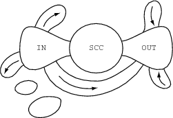This so-called bow-tie diagram is based on a snapshot of the web taken in May, 1999. The circle in the middle (the knot of the bow tie) is labeled SCC because it’s the largest strongly connected component of the web graph, consisting of some 56 million nodes. The left side of the bow, labeled IN, is the set of nodes not in the SCC but connected to a page in the SCC by some path; it contains about 44 million pages. The right side of the bow, OUT, is a set of pages with the following property: any node in OUT can be reached by following hyperlinks starting from any page in SCC, but no page in the SCC can be reached by following hyperlinks starting from a page in OUT.

Other interesting pieces of the web graph appear in the bow-tie diagram: tendrils that lead out to “nowhere” starting from IN or start at “nowhere” and lead into OUT, or that tunnel from IN to OUT without hitting SCC. There are also completely disconnected pieces (the separate blobs). Since someone adding a hyperlink to a page expresses interest in that page, one can infer that pages that aren’t pointed to either don’t interest anyone or haven’t yet been discovered. Pages in SCC exist in a complex tangled web of references. The IN pages are interested in the SCC but no one in the SCC is interested in them; just the opposite for OUT pages.

And, of course, the bow-tie diagram is based on a snapshot at a particular moment in time; the web is evolving quickly to reflect the changing interests of people all over the world. It used to be that people created most of the pages on the web by writing HTML. Today more pages on the web are created by programs than are written by humans, but even so many of the most interesting and most visited web pages have human authors. More than ever the web is a human creation reflecting human wants, needs, hopes and dreams; it’s as hard to predict what it will become as to predict what we will become.

13.5  Pianos and robots

But we’ve strayed beyond graphs and graphs algorithms and, as I mentioned, we’ll return in Chapter 14 to investigate the technology (and, to some extent, the psychology) that makes the World Wide Web possible. Before we leave the subject, I want to look at one more application involving graphs.

One summer day while I working on this chapter and looking for some interesting examples of applications involving graphs and graph algorithms, I had to interrupt my work to meet someone from the Neuroscience Department and go pick up a robot armthey were letting us use. I had asked a student by the name of Albert, an undergraduate working at Brown for the summer, to help me move the arm from Neuroscience to the Computer Science Department. The arm was a very nice multi-jointed arm with an industrial-quality controller and a force-torque sensor for the wrist joint that had never been installed (the force-torque sensor lets the arm detect when it hits something or sense the weight of an object held by its gripper). This arm was described as having six degrees of freedom, meaning that it had six different joints, each capable of turning independently of all the others.

The arm weighed around 40 kilograms (that’s around 88 pounds for the metrically challenged) and the controller about half that. In addition, we had to move the heavy table that the robot was mounted on and a bunch of crates and miscellaneous boxes. It was a good hour’s sweaty work but made interesting by having to figure out how to use the ancient (and woefully undersized by modern standards) freight elevator in the Neuroscience building and maneuver heavy and ungainly objects through doors and corridors.

I explained to Albert that our task was an instance of the general piano-movers problem, a problem in computational geometrythat involves moving an object, represented in terms of a set of coordinates and surfaces in three-dimensional space, from an initial location to a final destination in an environment containing other objects also represented in terms of points and surfaces. The objective is to find a path from the initial to the final location such that the object to be moved doesn’t intersect (collide) with the objects in the environment. Some human beings (piano movers in particular) are pretty good at this. This sort of thing is also important in robotics; think of planning a path for a mobile robot through a crowded room or for an assembly-line robot reaching into a partially assembled automobile to drill a hole or attach a part.

One elegant method of solving such problems involves reformulating them in a higher-dimensional space with one dimension for each degree of freedom. In general, a degree of freedom corresponds to the ability to move in a particular direction, for example, back and forth along some axis (also called a translational degree of freedom) or circularly around some axis (a rotational degree of freedom). Using an idea generally attributed to Tomás Lozano-Pérez, you can “shrink” the object to be moved and “grow” the objects to be avoided to obtain an equivalent problem in which the object to be moved is a point. The resulting formulation, called a configuration space, can then be “discretized” by carving up the space into a bunch of smaller regions.

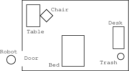
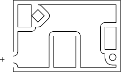
A simple example will help visualize this. Suppose you have a mobile robotthat looks like a trash can (remember R2D2 in “Star Wars”?). This shape is convenient, since we’ll assume that the robot can move in any direction in the horizontal plan and looks the same (a circle) from any angle when viewed from above. Let’s say this robot is supposed to go into your room, find your trash can and empty it. The first thing it has to do is plan a path from the door of your room to the trash can. To simplify things, we won’t worry about the z-axis (the height of the robot) but only the x- and y-axes (the floor of your room). The robot has two degrees of freedom, translation in the x and y directions. Suppose that you have a drawing of your bedroom showing your bed, desk, chairs, etc. — everything that might be an obstacle to a robot trying to maneuver there. Here’s a picture of the room with our robot standing just outside the door.

Now we grow the all of the obstacles, including the walls, by the radius of the trash-can-shaped robot, so that we can shrink the robot to a point. The next picture shows the result. The area enclosed by the curved line is called “free space” and indicates that portion of the room in which the robot can move without bumping into things.

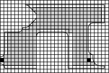
In the next drawing I’ve penciled in a grid over the room sketch. This is the first step in discretizing the problem. Next, I filled in the little square cells of the grid with gray if the area covered by a grid cell is more than 90% free space, and otherwise left it white. I’ve also marked the starting and target locations for the robot by coloring the corresponding cells black.

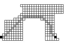
By laying down the grid over the continuous lines of the original drawing, I transformed a geometric problem to a problem involving graphs that I can solve with a path-finding algorithm. Where’s the graph? Nodes correspond to the cells designated as free space in the drawing above and links are defined as adjacency in the grid: there’s a link from one cell to another if the two cells are adjacent in the grid in any of the four compass directions or in any of the four diagonal directions. This last drawing, showing only the cells in free space, depicts a path (in gray) from the starting location to the target location that can easily be found using breadth-first search.

This same idea works for all kinds of robot shapes (not just trash-can shapes), in three dimensions of physical space as well as two, and with robots having many degrees of freedom, though the problems are harder computationally with many degrees of freedom. The computational effort also depends on how finely your grid divides up the space. The graph produced using this method is said to be of size exponential in the number of degrees of freedom. If you slice up the space using, say, 1000 lines along each dimensional axis, which is not uncommon, and you want to plan paths for a robot like the one Albert and I moved, then you’ll have a graph with (10³)⁶ or 10¹⁸ (1,000,000,000,000,000,000) nodes. Solving problems of this size requires more sophisticated algorithms and data structures than we’ve considered so far, but you can bet that trees and graphs play an important role.

You’ll encounter graph algorithms in every branch of computer science and the basic algorithms should be in the repertoire of every programmer. For a nice balance of theoretical analysis and practical algorithms I recommend Shimon Even’s Graph Algorithms. Most general algorithms textbooks, for example Cormen, Leiserson, Rivest and Stein’s Introduction to Algorithms, include substantial sections devoted to graph algorithms.