Lecture 10: Caching
» Lecture video (Brown ID required)
» Lecture code
» Post-Lecture Quiz (due 6pm Monday, March 2).
Caching
Last time, we looked at caching, where a small amount of fast storage speeds up access to a larger amount of slow storage. One reasonable question is what we actually mean by "fast storage" and "slow storage", and why need both. Couldn't we just put all of the data on our computer into fast storage?
To answer this question, it helps to look at what different kinds of storage cost and how this cost has changed over time.
The Storage Hierarchy
When we learn about computer science concepts, we often talk about "cost": the time cost and space cost of algorithms, memory efficiency, and storage space. These costs fundamentally shape the kinds of solutions we build. But financial costs also shape the systems we build, and the costs of the storage technologies we rely on have changed dramatically, as have their capacities and speeds.
The table below gives the price per megabyte of different storage technology, in price per megabyte (2010 dollars), up to 2019. (Note that flash/SSD storage did not exist until the early 2000s, when the technology became available.)
| Year | Memory (DRAM) | Flash/SSD | Hard disk |
|---|---|---|---|
| ~1955 | $411,000,000 | $6,230 | |
| 1970 | $734,000.00 | $260.00 | |
| 1990 | $148.20 | $5.45 | |
| 2003 | $0.09 | $0.305 | $0.00132 |
| 2010 | $0.019 | $0.00244 | $0.000073 |
| 2019 | $0.0029 | $0.000080 | $0.0000187 |
(Prices due to John C. McCallum, and inflation data from here. $1.00 in 1955 had "the same purchasing power" as $9.62 in 2019 dollars.)
Computer technology is amazing – not just for what it can do, but also for just how tremendously its cost has dropped over the course of just a few decades. The space required to store a modern smartphone photo (3 MB) on a harddisk would have costs tens of thousands of dollars in the 1950s, but now costs a fraction of a cent.
But one fundamental truth has remained the case across all these numbers: primary memory (DRAM) has always been substantially more expensive than long-term disk storage. This becomes even more evident if we normalize all numbers in the table to the cost of 1 MB of harddisk space in 2019, as the second table below does.
| Year | Memory (DRAM) | Flash/SSD | Hard disk |
|---|---|---|---|
| ~1955 | 219,800,000,000,000 | 333,155,000 | |
| 1970 | 39,250,000,000 | 13,900,000 | |
| 1990 | 7,925,000 | 291,000 | |
| 2003 | 4,800 | 16,300 | 70 |
| 2010 | 1,000 | 130 | 3.9 |
| 2019 | 155.1 | 4.3 | 1 |
As a consequence of this price differential, computers have always had more persistent disk space than primary memory. Harddisks and flash/SSD storage are persistent (i.e., they survive power failiures), while DRAM memory is volatile (i.e., its contents are lost when the computer loses power), but harddisk and flash/SSD are also much slower to access than memory.
In particular, when thinking about storage performance, we care about the latency to access data in storage. The latency denotes the time it takes until data retrieved is available if read, or until it is on the storage medium if written. A longer latency is worse, and a smaller latency better, as a smaller latency means that the computer can complete operations sooner.
Another important storage performance metric is throughput (or "bandwidth"), which is the number of operations completed per time unit. Throughput is often, though not always, the inverse of latency. An ideal storage medium would habe low latency and high throughput, as it takes very little time to complete a request, and many units of data can be transferred per second.
In reality, though, latency generally grows, and throughput drops, as storage media are further and further away from the processor. This is partly due to the storage technologies employed (some, like spinning harddisks, are cheap to manufacture, but slow), and partly due to the inevitable physics of sending information across longer and longer wires.
The table below shows the typical capacity, latency, and throughput achievable with the different storage technologies available in our computers.
| Storage type | Capacity | Latency | Throughput (random access) | Throughput (sequential) |
|---|---|---|---|---|
| Registers | ~30 (100s of bytes) | 0.5 ns | 16 GB/sec (2x10⁹ accesses/sec) | |
| SRAM (processor caches) | 5 MB | 4 ns | 1.6 GB/sec (2x10⁸ accesses/sec) | |
| DRAM (main memory) | 8 GB | 60 ns | 100 GB/sec | |
| SSD (stable storage) | 512 GB | 60 µs | 550 MB/sec | |
| Hard disk | 2–5 TB | 4–13 ms | 1 MB/sec | 200 MB/sec |
This notion of larger, cheaper, and slower storage further away from the processor, and smaller, faster, and more expensive storage closer to it is referred to as the storage hierarchy, as it's possibly to neatly rank storage according to these criteria. The storage hierarchy is often depicted as a pyramid, where wider (and lower) entries correspond to larger and slower forms of storage.
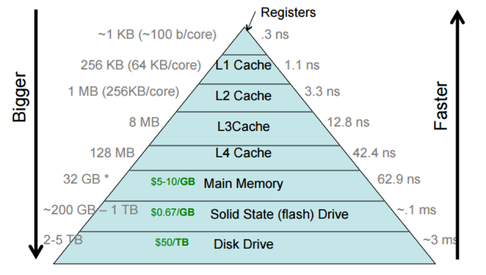
This picture includes processor caches, which are small regions of fast (SRAM) memory that are on the processor chip itself. The storage hierarchy shows the processor caches divided into multiple levels, with the L1 cache (sometimes pronounced "level-one cache") closer to the processor than the L2, L3, and L4 caches. This reflects how processor caches are actually laid out, but we often think of a processor cache as a single unit.
Different computers have different sizes and access costs for these hierarchy levels; the ones in the table above are typical. Here are some more, based on Malte's MacBook Air from ca. 2013: a few hundred bytes of of registers; ~5 MB of processor cache; 8 GB primary memory; 256 GB SSD. The processor cache divides into three levels: 128 KB of total L1 cache, divided into four 32 KB components; each L1 cache is accessed only by a single processor core (which makes it faster, as cores don't need to coordinate). There are 256 KB of L2 cache, and there are 4 MB of L3 cache shared by all cores.
Each layer in the storage hierarchy acts as a cache for the following layer.
Cache Structure
A generic cache is structured as follows.
The fast storage of the cache is divided into fixed-size slots. Each slot can hold data from slow storage, and is at any point in time either empty or occupied by data from slow storage. Each slot has a name (for instance, we might refer to "the first slot" in a cache, or "slot 0"). Slow storage is divided into blocks, which can occupy cache slots (so the cache slot size and the slow storage block size ought to be identical).
Each block on slow storage has an "address" (this is not a memory address! Disks and other storage media have their own addressing schemes). If a cache slot (in fast storage) is full, i.e., if it holds data from a block in slow storage, the cache must also know the address of that block.
In the contexts of specific levels in the hierarchy, slots and blocks are described by specific terms. For instance, a cache line is a slot in the processor cache (or, sometimes, a block in memory).
Cache Hits and Misses
Read caches must respond to user requests for data at particular addresses. On each access, a cache typically checks whether the specified block is already loaded into a slot. If it is, the cache returns that data; otherwise, the cache first loads the block into some slot, then returns the data from the slot.
A cache access is called a hit if the data accessed is already loaded into a cache slot, and can therefore be access quickly, and it's called a miss otherwise. Cache hits are good (they imply fast access), and cache misses are bad: they incur both the cost of accessing the cache and the cost of accessing the slower storage. Ideally, most accesses to the cache should be hits! In other words, we seek a high hit rate, where the hit rate is the fraction of accesses that hit.
For example, consider the arrayaccess.cc program. This program generates an in-memory array
of integers and then iterates over it, summing the integers, and measures the time to complete this iteration.
./arrayaccess -u -i 1 10000000 runs through the array in linear, increasing order
(-u), completes one iteration (-i 1), and uses an array of 10 million integers (ca.
40 MB).
Given that the array is in primary memory (DRAM), how long would we expect this to take? Let's focus on a
specific part: the access to the first three integers in the array (i.e., array[0] to
array[2]). If we didn't have a cache at all, accessing each integer would incur a latency of 60
ns (the latency of DRAM access). For the first three integers, we'd therefore spend 60 ns + 60 ns + 60 ns =
180 ns.
But we do have the processor caches, which are faster to access than DRAM! They can hold blocks from DRAM in their slots. Since no blocks of the array are in any processor cache at the start of the program, the access to the first integer still goes to DRAM and takes 60 ns. But this access will fetch a whole cache block, which consists of multiple integers, and deposit it into a slot of the L3 processor cache (and, in fact, the L2 and L1, but we will focus this example on the L3 cache). Let's assume the cache slot size is 12 bytes (i.e., three integers) for the example; real cache lines are often on the order of 64 or 128 bytes long. If the first access brings the block into the cache, the subsequent accesses to the second and third integers can read them directly from the cache, which takes about 4 ns per read for the L3 cache. Thus, we end up with a total time of 60 ns + 4 ns + 4 ns = 68 ns, which is much faster than 180 ns.
The principle behind this speedup is called locality of reference. Caching is based on the
assumption that if a program accesses a location in memory, it is likely to access this location or an
adjacent location again in the future. In many real-world programs, this assumption is a good one, as it
is often true. In our example, we have spatial locality of reference, as access to
array[0] is indeed soon after followed by accesses to array[1] and
array[2], which are already in the cache.
By contrast, a totally random access pattern has no locality of reference, and caching generally
does not help much with it. With our arrayaccess program, passing -r changes the
access to be entirely random, i.e., we still access each integer, but we do so in a random order. Despite the
fact that the program sums just as many integers, it takes much longer (on the order of 10x longer) to run!
This is because it does not benefit from caching.
Cache Replacement
In our nice, linear arrayaccess example, the first access to the array brought the first block
into the processor caches. Once the program hits the second block, that will also be brought into the cache,
filling another slot, as will the third, etc. But what happens once all cache slots are full? In this situation,
the cache needs to throw out an existing block to free up a slot for a new block. This is called cache
eviction, and the way the cache decides which slot to free up is called an "eviction policy" or a
"replacement policy".
What might a good eviction policy be? We would like the cache to be effective in the future, so ideally we want to avoid evicting a block that we will need shortly after. On option is to always evict the oldest block in the cache, i.e., to cycle through slots as eviction is needed. This is a round-robin, or first-in, first-out (FIFO) policy. Another sensible policy is to evict the cache entry that was least recently accessed; this is a policy called least recently used (LRU), and happens to be what most real-world caches use.
But what's the best replacement policy? Intuitively, it is a policy that always evicts the block that will be accessed farthest into the future. This policy is impossible to implement in the real world unless we know the future, but it is provably optimal (no algorithm can do better)! Consequently, this policy is called Bélády's optimal algorithm, named after its discoverer, László Bélády (the article).
It turns out that processors can sometimes make good guesses at the future, however. Looping linearly over a
large array, as we do in ./arrayaccess -u, is such a case. The processor can detect that we are
always accessing the neighboring block after the previous one, and it can speculatively bring the next block into
memory while it still works on the summation for the previous block. This speculative loading of blocks into the
cache is called prefetching. If it works well, prefetching can remove some of the 60 ns price of the first
access to each block, as the block may already be in the cache when we access it!
Measuring Actual Cache Performance
We can see the cache in action by running our ./arrayaccess program under a tool that reads
information from special "performance counter" registers in the processor. The perf.sh
script invokes this tool and sets it to measure the last-level cache (LLC) accesses ("loads") and
misses. In our example, the L3 cache is the last-level cache.
When we run ./arrayaccess -u -i 1 10000000, we should expect a hit rate smaller than 100%,
since the first access to each block triggers a cache miss. Sometimes, but not always, prefetching manages to
ensure that the next block is already in the cache (which increases the hit rate); the precise numbers depend
on a variety of factors, including what else is running on the computer at the same time.
For example, we may get the following output:
$ ./perf.sh ./arrayaccess -u -i 1 10000000
accessing 10000000 integers 1 times in sequential order:
[0, 1, 2, 3, 4, 5, 6, 7, 8, 9, 10, 11, 12, 13, 14, 15, 16, 17, 18, 19, ...]
OK in 0.007934 sec!

 Performance counter stats for './arrayaccess -u -i 1 10000000':

           307,936      LLC-misses                #   25.67% of all LL-cache hits
         1,199,483      LLC-loads

       0.048342578 seconds time elapsed
This indicates that we experienced a roughly 74% cache hit rate (100% mius the 26% miss rate) – a rather decent result.
If we instead run the arrayaccess program with a random access pattern, the hit rate is much
lower and there are more misses:
$ ./perf.sh ./arrayaccess -r -i 1 10000000
accessing 10000000 integers 1 times in random order:
[4281095, 3661082, 3488908, 9060979, 7747793, 8711155, 427716, 9760492, 9886661, 9641421, 9118652, 490027, 3368690, 3890299, 4340420, 7513926, 3770178, 5924221, 4089172, 3455736, ...]
OK in 0.152167 sec!

 Performance counter stats for './arrayaccess -r -i 1 10000000':

        19,854,838      LLC-misses                #   78.03% of all LL-cache hits
        25,443,796      LLC-loads

       0.754197032 seconds time elapsed
Here, the hit rate is only 22%, and 78% of cache accesses result in misses. As a result, the program runs 16x slower
than when it accessed memory sequentially and benefited from locality of reference and prefetching.
Summary
Today, further developed our understand of caches, why they are necessary, and why they benefit performance. We saw that differences in the price of storage technologies create a storage hierarchy with smaller, but faster, storage at the top, and slower, but larger storage at the bottom. Caches are a way of making the bottom layers appear faster than they actually are!
We discussed how caches are made from slots that can holds blocks of data from lower levels in the storage hierarchy, and we looked at the specific example of processor caches to illustrate this. We found that accessing data already in the cache (a "hit") is much faster than accessing it on the underlying storage to bring the block into the cache (a "miss"). We also considered different algorithms for which slot to free up when the cache is full and a new block needs to be brought into the cache, and found the widely-used LRU algorithm as a reasonable predictor of future access patterns due to the locality of reference exhibited by typical programs.
There is a lot more to say about caches, and you will learn some more in Lab 4. We will also talk about caches again in the context of distributed systems later in the course!