Final Project - Image Morphing

The basic procedure for image morphing is as follows:

• Select corresponding points
• Warp one set of points towards another and vice versa
• Blend the results of the warping

Selecting points

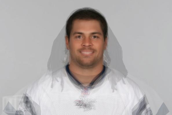
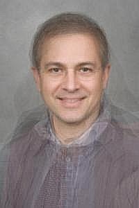
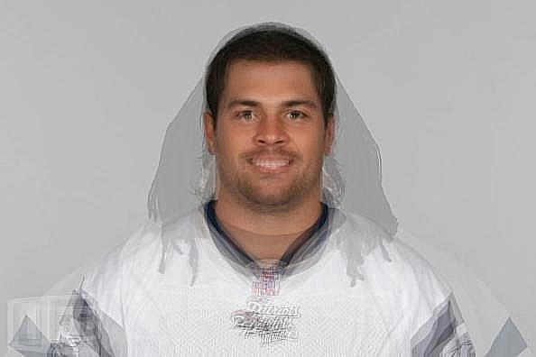
Deciding what points to select is a nontrivial matter. If given more time, I might have attempted to implement a feature detection system to algorithmically select the points. However, since my focus was on the actual morphing, I manually selected points. For a given image set I selected the same number of points in the same order for each image in the set (or pair). These points were more or less distributed throughout the regions of expected warping at points which would be easily identifiable across different images based on a simple set of rules. For example, point 26 and 27 for the face warping corresponded the centers of the left and right eyes respectively. Shown below are some examples of the points used for certain images.

In some cases, choosing the wrong points caused issues. For example, if the chosen feature when out of view or crossed some other feature such that the triangles were no longer in the same order, the warping no longer worked as well. This was especially true in my attempts to use image warping to show animation. In the example below, the first two images warp fine, however, the third and fourth do not work as well.

Warping

The actual warping of an image is a matter of determining and applying a spatial transformation based on the pairs of control points. There are of course a variety of different methods to achieve this. In my implementation, I chose to use a local weighted mean which has the benefit of accounting for distortion which varies locally. Since I figured that different facial features would vary differently from one face to the next (eg. larger nose but smaller eyes) I decided that this would be the best choice for determining the transform to apply. To actually create the transform I used the MATLAB function cp2tform, which follows the following basic algorithm for the local weighted mean:

for each control point
	neighbors = the 12 closest control points
	use neighbors and their corresponding pairs to infer a second-order polynomial
	radius of influence = center point - furthest neighbor				

The triangles connecting the points on the images shown earlier were the result of finding the Delaunay triangulation, which in some cases may be used to infer an affine mapping between the two set of points. I ultimately decided to use a higher order polynomial rather than the linear affine transform since the method using the Delaunay triangulation placed more restrictions upon the points used which made it more difficult to run when using certain image sets. The results from either method are shown below for comparison.

local weighted mean	piecewise linear

Using image morphing

Transistions

for i = 1:n
	for each point p in the original image and point q in the second image
		new_p = p +(1-i/n)*(q-p)
	new_p is then warped towards q

Image morphing can be used to transistion smoothly through a set of images. The basic idea is to morph each image in the list towards the next one. In this case, the process is really just a matter of putting the results from morphing a pair of images in the correct order.

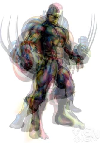
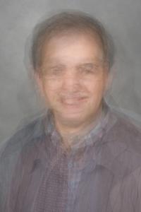
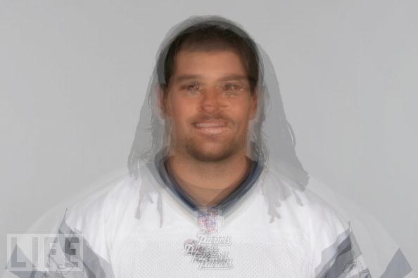
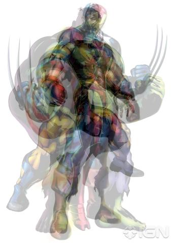
I also tried to see how well morphing would work with images that were not very similar at all.

Average

Image morphing may also be used to compute the average of multiple images. In this case, the desired output is a single frame, so it is not necessary to specify the number of steps. The general procedure is to compute the average set of points for the images. Given this average set of points, warp each image towards that average and then blend the results.
I then applied a sharpening filter to these results to see if I could produces a more convincing image.
Shown below are the results from just simple averaging alone.