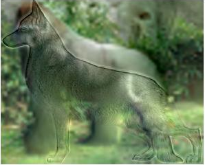
What is Filtering?
Filtering is a process where we modify pixel data to change the appearance of an image. Filters can do all sorts of things, including blurring, sharpening, edge detection, and many more operations. Filtering is often used as a synonym for convolution, and although there is a slight difference, for our purposes, they are identical terms. An image can be modled as an mxn grid of pixel data. For simplicty, we can assume our images are gray-scale and for each pixel have only an intensity value between 0 and 1.
To filter an image we first need a filter. A filter is an array smaller than the image. Often this array is symetric and square. Like our image which is an mxn grid of numbers, the filter is often represented as a jxk grid of numbers as well. The sum of all numbers in a filter often adds to 1, which means that overall the image preserves its brightness.
Let I be the original image, I' be a filtered image, and F be our filter. To find the value of the pixel (x,y) in I', represented I'(x,y). We center our filter over the pixel I(x,y). Then I'(x,y) = SUM( F * I), where for each pixely (a,b) that F lies on top of, we multiply I(a,b) * F(u,v), where F(u,v) is the value of the filter above (a,b). To create I' we repeat this process for all x and y. Here is an example (the values are intergers for simplicity): Let I = [4, 8, 4, 16, 20, 4] and F = [.25, .5, .25]:Then I' = [*, 6, 8, 14, 15, *].
Note that the reason there are * in the boundaries is because we did not discuss what to do when the filter falls off the end of the image. There are many ways to deal with this. Sometimes "out of range" pixels are given value 0, other times the edge is copied. Most often, we treat pixels off the edge as having a symetric reflection over that edge.
A Closer Look at the Gaussian Filter & the Frequency Domain
A Gaussian filter is based off of the Gaussian function: a*e^[-x^2 / (2c^2)]. The Gaussian function has a characteristic bell curve shape. For filtering we are concerned about the two dimensional version of the gaussian function which looks like:
An excellent blurring filter can be constructed based on this function. (Interestingly, a 2-D Gaussian filter can be constructed from subsequent passes of a horizontal and vertical Gaussian filter, which increases the simplicity and speed of code, but the 2-D filter is easier to understand intuitively). We can understand why this function blurs by examining its shape. For each pixel, it will reset its value to a weighted averaging of its own value and its surrounding neighbors.
Another way to think of the Gaussian is to consider the image in its frequency domain. Rather than thinking of an image as discrete pixels, we can instead think of it as a continuous intensity signaled that has been sampled at specified regual intervals, such that the viewer still has a pretty good perception of the original signal. For example, if you had the signal y = x, and sampled at intervals of .1 from x = 0 to 1, you would get: [0, .1, .2, .3, .4, .5, .6, .7, .8, .9, 1.0], which is enough to give you the general idea of what the continuous signal looks like from x = 0 to 1. Every signal can be constructed as a sum of weighted sines and cosines with varying frequencies. This process can be done using the Forier Transform, but the specifics of this transformation are not necessary to understand hybrid images. The new function in the frequency domain is known as the dual of the original signal. When we filter (or convolve) in the spatial domain, it is the equivalent of multiplying the dual of the image with the dual of the filter in the frequency domain. Interestingly, the dual of a gaussian is another gaussian. The center of the gaussian in the frequency domain is aligned with the lowest frequency, so when we multiply the signal by the gaussian, we are effectively removing all high frequency signals. Thus we know that a blurred image is the same as an image with the high frequencies removed.
