Sondik's One-Pass Algorithm

The next algorithm we discuss was actually the first exact POMDP algorithm proposed and is due to Sondik (1971). This algorithm starts with an arbitrary belief point, constructs the vector for that point and then defines a set of constraints over the belief space where this vector is guaranteed to be dominant.

The region defined is actually the intersection of three easier to describe regions. When we construct a vector from a belief point b we know what is the strategy that vector represents. This strategy is the best one for that belief point and some nearby belief points. However, it might not be the best strategy for all belief points. There are two ways that this strategy might not be the best strategy: either the immediate action doesn't change and the future strategy changes; or another action might become better. The first region assures that even if the best action doesn't change, the future course of action doesn't change either.

Sondik's first region

The second region assures that the best vector for the current action is not exceeded by each of the current best vectors for each of the other actions. This says that even though some action a' and future course of action isn't as good as a at the point b, there could be a very close point where that action and course of action becomes better.

Sondik's second region

Finally, it may be that a_1 and a future course of action will never be better that the current best action and its best future course of action. However, a_1 and another course of action may become better than the current best action and its course of action. We need to restrict the region to incorporate this. We do this be defining the limits of each action's best region.

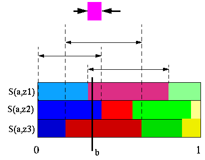
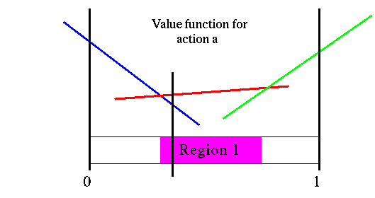
The figure below shows the value function for action a and the first region we defined above.

Sondik's first region and value function

We now superimpose the value for the other action (shown in dashed lines).

Sondik's second region

The dashed red line is the best vector for this other action at belief point b, but it is not as good at the belief point b. Note that there are belief states where this vector is better. This second set of constraints assures that we restrict ourselves to the region where the current best action remains the best action. You can see from the picture that the first region by itself would include points where the solid red line vector was not the best value attainable.

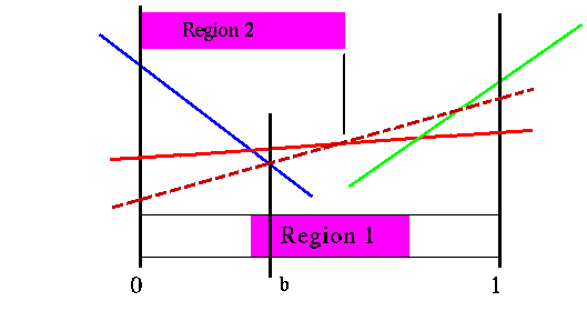
The dashed red line represents a particular future strategy for the non-optimal action. In other words, the best strategy to do if we were force to take that action first. The above region makes sure we restrict ourselves to belief points where this strategy is not better than what we have at belief point b. However, The final region is for the case where not only does the best action change, but the best strategy for that other action changes from what is the current best strategy. The dashed red line only shows part of the story for what is happening for the other action. We know that the dashed red line represents the best future strategy for that action at point b, but we know nothing about other future strategies for that action.

To ensure that we restrict ourselves to belief points where the action and future strategy doesn't change, we need to include the region where the dashed red line is the best strategy for the other action. This figure shows all the different strategies for the other action, though there are only two in this example.

Sondik's third region

The region where the red dashed line dominates the blue dashed line is the third region. The intersection of the three regions is the region where we are assured that the solid red vector is the best one. However, note that we are being too restrictive here. The points to the left of b still have the solid red vector as the best one. But because of the third region we cannot include those in the region.

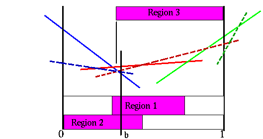
The following figure shows the complete region that is imposed by Sondik's one-pass algorithm. It is the intersection of the three regions previously described.

Complete Sondik region

With this region defined we can use linear programming to find a point on the edge of this region. The useful part of this point is that it also lies on the boundary of a region adjacent to the current region. In effect, it gives us a point in another region.

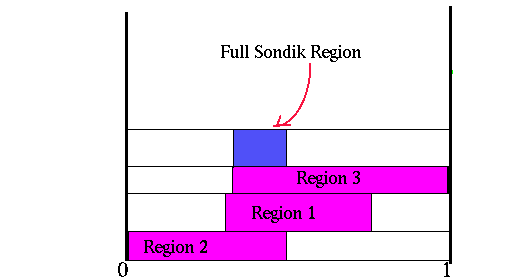
Unfortunately, the regions defined by Sondik's algorithm are extremely conservative. These are not guaranteed to be the complete region where the vector is dominant as we saw in the last figure. Thus we might find that we generate the same vector for many belief points.

Continue

Back | POMDP Tutorial | Next