

In this section we finally start to get to the heart of the matter. We will start to introduce the graphical representation we use and then explain how we can use the value iteration algorithm to solve a POMDP problem. Once this is established, we can delve into the particular algorithms that have been used to solve POMDPs.
In CO-MDPs our problem is to find a mapping from states to actions; in POMDPs our problem is to find a mapping from probability distributions (over states) to actions. We will refer to a probability distribution over states as a belief state and the entire probability space (the set of all possible probability distributions) as the belief space.
The figure below introduces how we will represent the belief space. To keep things as simple as possible, we will use a two state POMDP as our running example. For a two state POMDP we can represent the belief state with a single number. Since a belief state is a probability distribution, the sum of all probabilities must sum to 1. With a two state POMDP, if we are given the probability for being in one of the states as being 'p', then we know that the probability of being in the other state must be '1-p'. Therefore the entire space of belief states can be represented as a line segment. The figure below shows this, though we have made the line segment have a significant width.

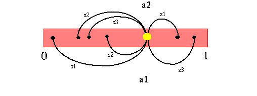
Let us go back to the updating of the belief state discussed earlier. Assume we start with a particular belief state b and we take action a1 and receive observation z1 after taking that action. Then our next belief state is fully determined. In fact, since we are assuming that there are a finite number of actions and a finite number of observations, given a belief state, there are a finite number of possible next belief states. These correspond to each combination of action and observation. The figure below shows this process graphically for a POMDP with two states (s1 and s2), two actions (a1 and a2) and three observations (z1, z2 and z3). The starting belief state is the big yellow dot and the resulting belief states are the smaller black dots. The arcs represent the process of transforming the belief state.

It turns out that the process of maintaining the belief state is Markovian; the next belief state depends only on the current belief state (and the current action and observation). In fact, we can convert a discrete POMDP problem into a continuous space CO-MDP problem where the continuous space is the belief space. The transitions of this new continuous space CO-MDP are easily derived from the transition and observation probabilities of the POMDP (remember: no formulas here). What this means is that we are now back to solving a CO-MDP and we can use the value iteration (VI) algorithm. However, we will need to adapt the algorithm some.
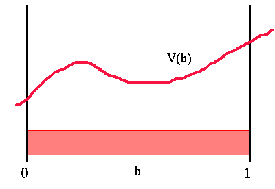
The big problem using value iteration here is the continuous state space. In CO-MDP value iteration we simply maintain a table with one entry per state. The value of each state is stored in the table and we have a nice finite representation of the value function. Since we now have a continuous space the value function is some arbitrary function over belief space. The figure below shows a sample value function over belief space. Here 'b' is a belief space and the value function, 'V(b)', is a function of 'b'. Thus our first problem is how we can easily represent this value function.

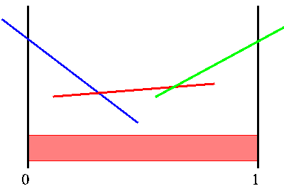
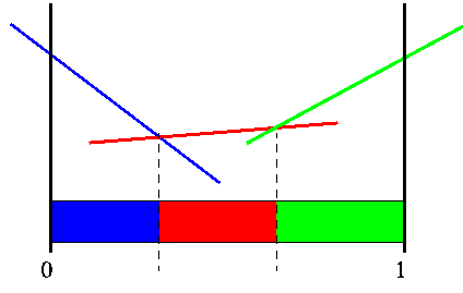
The figure below shows a sample value function over belief space for a POMDP. It is the upper surface of a finite number of linear segments. We have colored the segments for a reason to be explained later.

We can now represent the value function for each horizon as a set of vectors. To find the value of a belief state, we simply find the vector that has the largest dot product with the belief state.
Instead of linear segments over belief space, another way to view the function is that it partitions belief space into a finite number of segments. We will be using both the value function and this partitioning representation to explain the algorithms. Keep in mind that they are more or less interchangeable.

Unfortunately, the continuous space causes us further problems. In each iteration of value iteration in the discrete state space, we would find a state's new value by looping over all the possible next states. However, for continuous state CO-MDPs it is impossible to enumerate all possible states (can you say "uncountably infinite"?).
This is the main obstacle that needs to be overcome and the specific algorithms described later are all different approaches to solve this difficulty. Once we overcome this difficulty, the problem is solved and value iteration works the same here as in the discrete CO-MDP case. The problem now boils down to one stage of value iteration; given a set of vectors representing the value function for horizon 'h', we just need to generate the set of vectors for the value function of horizon 'h+1'
