Mathematics of stitching
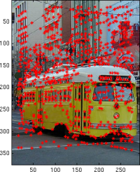
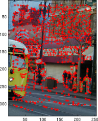
Being able to align and composite images means we need to understand where their features correspond. I used the Harris corner detector on each image as the first step in this process. Harris works by finding corner-like features in the gradient domain, and returns us the coordinates and "strength" of each feature it finds. One assumption here is that Harris will find the salient features that correspond between images; if this doesn't work, we're out of luck. That means some amount of success will depend on how the photographer overlapped his shots, and whether there are enough unique and corner-like features in the overlap.
Adaptive non-maximal suppression. The Harris detector has some local non-maximum suppression: no more than one feature will exist in any [3 3] window. But we want fine-grained control over the number of points returned, and we want to ensure we have a spatially diverse set of feature points. To get this, I implemented the ANMS algorithm described in "Multi-Image Matching using Multi-Scale Oriented Patches" (Brown, Szeliski and Winder). This works by computing the suppression radius for each feature (strongest overall has radius of infinity), which is the smallest distance to another point that is significantly stronger (based on a robustness parameter). After the strongest point, every other feature will have a non-negative radius at most as big as its distance from the strongest. We can then sort our features based on radius size, and pull the first n features when we request a specific amount. In doing this, we aren't guaranteed to get the n features with the highest corner strengths, but instead, we get the n most dominant in their region, which ensures we get spatially distributed strong points.
 | 
|
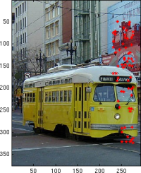
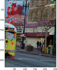
Feature matching with descriptors. The next step is to associate features across images. Humans do this very well, even with substantial noise or transformations between images. Our approach in automating this will be to compute a descriptor at each feature point that encodes information about colors around it, as in the Brown paper. In this case, we aren't worrying about rotation or scale variations, but these are things we ought to take care of in a robust vision system. For my descriptors, I measure 64 colors (8x8 grid) around the feature, with spacing 3 between each. I scale down images with low-pass filtering, then look at adjacent pixels as a way to sample these colors without aliasing. Each descriptor is standardized to be zero-mean and is divided by its standard deviation.
I use the provided dist2 function to compare descriptors across images, then look for strongest matches from one image into the other. One critical step is that we want to reject features that match closely with multiple other features. These are more likely to be outliers than other feature matches, because they may indicate texture or repeated scene objects that our descriptor footprint isn't large enough to identify uniquely. I use Lowe's method of thresholding on e1_nn / e2_nn, which is the ratio of a feature's best match score (lower is better) to its second best match score. In my implementation, I reject features whose ratios are higher than 0.5 and get good results.
 | 
|
Robustly recovering homographies. We have a mapping between features in each image. How do we build a panorama from these? The main idea is that we can recover a projective transformation (i.e. homography) that take a point in the second image and returns its location in the space of the first image. Applying this to all points in the second image, we now know where to composite the images.
Paul Heckbert's Projective Mapping for Image Warping guide covers the mathematics of computing a homography from four correspondence features. We can use that construction to sample point-sets from our matches, evaluating the homography it yields and iterating to find the lowest error homography. I implemented RANSAC to do this, with 2000 iterations, a minimum consensus of 10, and an error threshold of one pixel (i.e. a 'consenting match' is recovered to within one pixel radius when applying a potential homography). Given that, we can composite our panorama using steps similar to those in Mikkel Stegmann's warping tutorial. I finish by using Poisson blending to composite the images to try and hide seams. Alpha blending or graphcut are likely to help disguise the seams as well, but I'll leave that for next time.
 | 
|