Steve Gomez (steveg) .
February 13, 2010
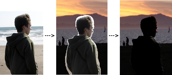
In this project, we blend images seamlessly by solving for unknown pixel colors using discrete Poisson equations. The pixel colors we want to transplant into an image will be unknown initially, because they will be adjusted (e.g. for color constancy, edges) if we want the composite image to look right. We form a system of linear equations describing these unknowns, using our known data (unmasked colors that are unchanged in the target image) and solve in Matlab.
|
Algorithm implementation
The blending constraints are given by the Perez paper ("Poisson Image Editing", in SIGGRAPH 2003). My approach is to move all unknowns to the left-side of the equations, forming a sparse matrix of coefficients for each of m*n pixels (in m*n target).
To be efficient, my implementation builds vectors that describe entries into the coefficient matrix, then constructs a sparse matrix at once before solving with left-division. The vectors (which correspond to row and column indices, and the corresponding entries) are preallocated to 5*m*n, which is an upper bound occurring when the entire target image is replaced. The number "5" comes from the maximum number of non-zero coefficients a given unknown has in its corresponding discrete Poisson constraint: 1 for itself, and -1 for up to four neighboring pixels. I fill these vectors iteratively, then use Matlab's sparse constructor, and left-divide with the "b" vector (known right-sides of the constraint equations) to get the image.
Each channel is built separately, then composited. My largest image (614x461 pix) blends and composites in about 5 seconds, and the smaller images are much faster.
Transparency/mixed gradient blending with Poisson
To add the mixed gradient blending the paper described, I check both source and target gradients when building the Poisson equations. More specifically, when previously we were adding the color difference between a pixel in the source and its neighbors, we now compute a difference at the same location in the target. When the background gradient is stronger at that pixel, we assume that value should be blended in instead of gradient at the source image.
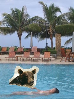
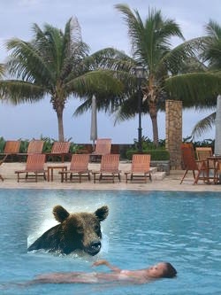
The mixed gradient approach doesn't always work because it sometimes adds transparency to objects that we know should be opaque. I tried to capture good and bad examples by computing frames with a timed offset, and exporting those as avi movies in Matlab.
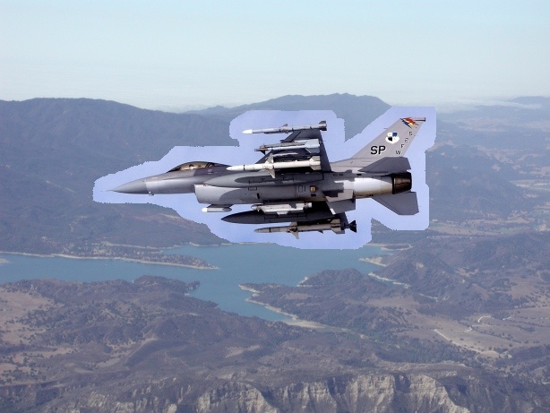
In all these videos, the common theme is that transparency creates much more believable boundaries at the source insertion, but it can cause problems when the background has high-frequency details under the mask location. In the bear videos, the border is noticably better with transparency, but the bear's head tends to show background details as it descends. In the jet videos, transparency did a very good job of removing the halo of blended colors as the jet crosses the mountain line.
The take-away lesson is that we need to pay attention both to scene semantics (i.e. "should a bear be transparent?") and high-frequency details under the mask if we want to use mixed gradient blending.
Laplacian pyramid blending
In Laplacian blending, we build a difference of Gaussians (DoG) pyramid for the source and target. Each level contains the frequencies not captured at coarser levels in the Gaussian pyramid. Given a Laplacian pyramid, we can also rebuild the original image by scaling up lower levels and adding in the Laplacian at each step.
To blend, we use pyramid levels of the mask to combine (with alpha blending) Laplacian levels of the source and target, creating a new Laplacian pyramid. When we 'reconstitute' the image from this pyramid, the lower frequencies will be blended and higher frequencies preserved.
| Cut and paste | Poisson blend | Laplacian |
|---|---|---|
| 
| |
| 
| |

| 
| |
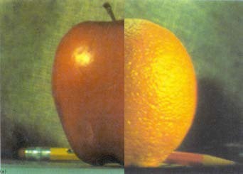
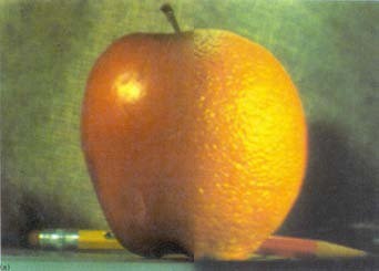
Here I show the apple/orange typically presented for Laplacian blending. One difference with this type of blending is that frequencies only blend as much as the mask is blurred/interpolated at a given level. So blending is usually localized near the mask boundaries (varying with the kernel size of the Gaussian -- here I use [100,100] in 2d). This is not necessarily true of Poisson blending, where masked pixels are determined by their neighbors (and transitively, by their neighbors).
Images
Blending with my own photos

| ||

| ||

| ||

| ||

|