
As our noble digital photographer ventures out into the wilderness armed with their trusted cameras, they are repeatedly hounded in their quest for truth by the vile and iniquitous Noise Monster. In this lab we will cover one of the tools the lionhearted photographer can use to combat this fiendish interloper: the bilateral filter.

If you have past experience with filtering, you may be aware of how it can be used to remove unwanted frequencies (a fancy term for noise) from an input signal. What, then, makes the bilateral filter so special? To appreciate the advantages offered by a bilateral filter, it would be useful to first understand why an old-fashioned Gaussian filter proves insufficient when it comes to processing images.
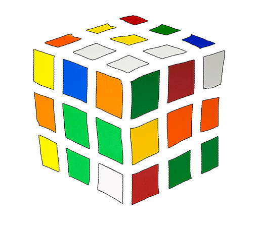
Let's load up a noisy image in Python and convolve it with a Gaussian filter:
    from PIL import Image
    import numpy as np
    from scipy import ndimage

    img = np.array(Image.open('path/to/rubiks_cube.png'), dtype=np.float32)
    img_filtered = ndimage.gaussian_filter(img, sigma=[3, 3, 0])

    Image.fromarray(img_filtered.astype(np.uint8)).show()


While the amount of noise has certainly been reduced, the astute viewer will notice that so has most of the detail around object edges. Everything appears blurry now. This is why a Gaussian—or any other convolutional filter, for that matter—is not very useful as a noise supression tool for images: it filters indiscriminately, leading to loss of resolution. What we want, instead, is a filter that works on the `internal' pixels of an object, but leaves the edges alone.
Q1: The following two figures show a crude decomposition of our image into edge (left) and non-edge regions (right). Do you notice anything different about the color composition of the regions in each case? How many different colors can you count in each region?

In class, we saw how the median filter can handle edge-aware filtering. Let us now see how a bilateral filter handles the same image.
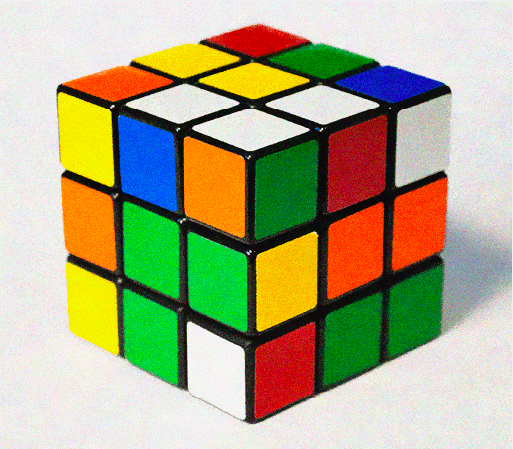
The result, in this case, is much closer to what we want.
Q2: Based on the color composition of the edge and non-edge regions shown above, what do you think the bilateral filter is doing?
The bilateral filter is a Gaussian that acts strongly on regions of uniform color, and lightly on regions with high color variance. Since we expect edges to have high color variance, the bilateral filter acts as an edge-preserving or edge-aware filter.
Let us dive into the details of how the bilateral filter works. Once again, the Gaussian distribution provides a good launching pad. First, let's remind ourselves of its 2D form—here unnormalized. Let's assume the Gaussian of variance \(\sigma\) is centered at a point \(p\) and we're sampling the PDF for a point at \(q\): \(q\) is \(d\) away from \(p\).
The Gaussian filter applied at a pixel index \(p\) in image \(I\) can be written as:
where \(I_q\) is the value at pixel index \(q\), and \(S\) denotes a small neighborhood
of pixels around \(p\). The \(\mathcal{N}\) denotes a Gaussian (which is also called a \(\mathcal{N}\)ormal
distribution), and \(w\) is the normalization factor—this preserves image brightness during filtering.
A simple Python implementation of this equation is provided in Listing 2. While this isn't the most efficient
implementation of Gaussian filtering—we would typically use a numpy implementation—it is helpful for understanding
the Gaussian filter and the changes we need to make to a Gaussian filter to obtain a bilateral filter.
Note: If you have trouble mentally mapping this code to your conceptual understanding of filtering, feel free to review the course slides on filtering.
# Gaussian convolution applied at each pixel in an image
  # Parameters:
  #   im: Image to filter, provided as a numpy array
  #   sigma:  The variance of the Gaussian (e.g., 1)
  #
  import numpy as np

  def gaussian(im, sigma):
      height, width, _ = im.shape
      img_filtered = np.zeros([height, width, 3])

      # Define filter size.
      # A Gaussian has infinite support, but most of it's mass lies within
      # three standard deviations of the mean. The standard deviation is
      # the square of the variance, sigma.
      n = np.int(np.sqrt(sigma) * 3)

      # Iterate over pixel locations p
      for p_y in range(height):
          for p_x in range(width):
              gp = 0
              w = 0

              # Iterate over kernel locations to define pixel q
              for i in range(-n, n):
                  for j in range(-n, n):
                      # Make sure no index goes out of bounds of the image
                      q_y = np.max([0, np.min([height - 1, p_y + i])])
                      q_x = np.max([0, np.min([width - 1, p_x + j])])
                      # Computer Gaussian filter weight at this filter pixel
                      g = np.exp( -((q_x - p_x)**2 + (q_y - p_y)**2) / (2 * sigma**2) )

                      # Accumulate filtered output
                      gp += g * im[q_y, q_x, :]
                      # Accumulate filter weight for later normalization, to maintain image brightness
                      w += g
              img_filtered[p_y, p_x, :] = gp / (w + np.finfo(np.float32).eps)

      return img_filtered
# Gaussian convolution applied at a pixel in an image
import numpy as np
from PIL import Image
import filt

img = np.array(Image.open('../img/rubiks_cube.png'), dtype=np.float32)
img_filtered = np.asarray(filt.gaussian(img, 3))
Image.fromarray(img_filtered.astype(np.uint8)).show()
Let's try to speed the code up a bit. We will do this using a python library called Cython. The main source of latency in our Python code of Listing 2 is the nested for loops. Cython allows us to run these as compiled C code, which is very fast. You can install Cython using Pip:
$> source ./../path/to/your/venv/bin/activate $> pip install cython The changes that we need to make to the python code from Listing 2 are shown in Listing 4:
exp and sqrt, andcdef to our variable definitions, and we strongly type our variables with int and double.
# Gaussian convolution applied at each pixel in an image (Cython version)
# Parameters:
#   im: Image to filter, provided as a numpy array
#   sigma:  The variance of the Gaussian (e.g., 1)
#

# Tell Cython to use the faster C libraries.
# If we add any additional math functions, we could also add their C versions here.
from libc.math cimport exp
from libc.math cimport sqrt

import numpy as np

def gaussian(float[:, :, :] im, double sigma):
    cdef int height = im.shape[0]  # cdef int tells Cython that this variable should be converted to a C int
    cdef int width = im.shape[1]   #

    # cdef double[:, :, :] to store this as a 3D array of doubles
    cdef double[:, :, :] img_filtered = np.zeros([height, width, 3])

    # A Gaussian has infinite support, but most of it's mass lies within
    # three standard deviations of the mean. The standard deviation is
    # the square of the variance, sigma.
    cdef int n = np.int(sqrt(sigma) * 3)

    cdef int p_y, p_x, i, j, q_y, q_x

    cdef double g, gpr, gpg, gpb
    cdef double w = 0

    # The rest of the code is similar, only now we have to explicitly assign the r, g, and b channels
    for p_y in range(height):
        for p_x in range(width):
            gpr = 0
            gpg = 0
            gpb = 0
            w = 0
            for i in range(-n, n):
                for j in range(-n, n):
                    q_y = max([0, min([height - 1, p_y + i])])
                    q_x = max([0, min([width - 1, p_x + j])])
                    g = exp( -((q_x - p_x)**2 + (q_y - p_y)**2) / (2 * sigma**2) )

                    gpr += g * im[q_y, q_x, 0]
                    gpg += g * im[q_y, q_x, 1]
                    gpb += g * im[q_y, q_x, 2]
                    w += g

            img_filtered[p_y, p_x, 0] = gpr / (w + 1e-5)
            img_filtered[p_y, p_x, 1] = gpg / (w + 1e-5)
            img_filtered[p_y, p_x, 2] = gpb / (w + 1e-5)

    return img_filtered
Every time we make changes to our code, and before we run our code, we must ask Cython to compile the changes we made.
We've set this up for you: download setup.py and execute the following command:
$> python setup.py build_ext --inplace
Try running $python our_gaussian.py now. You should see a significant improvement in speed.
You can do this for any Python code. Sometimes it's impossible to vectorize code into numpy functions. Cython gives us another option to make Python code faster.
In Equation 1, the contribution of each Iq to the filtered value of p, G(p), is determined by the distance between pixel p and q, that is, |p -q|. To preserve detail around edges, we would like to add an additional term to Equation 1 that accounts for the color variance around p as well.
It turns out that one controllable way to modulate filtering in edge regions is to weight the contribution of each Iq to G(p) in Equation 1 by the color difference between p and q.

Now, let's go a step farther, and weight the color difference based on a Gaussian.
Congratulations! You have successfully implemented a bilateral filter:
Since the standard definition uses a Gaussian as the weight decay function, bilateral filters are commonly defined by the variance values of the two Gaussians that determine the weights: \(\textrm{BF}(\sigma_1, \sigma_2)\). This is what makes them powerful controllable edge-aware filters through varying these sigma values. We will see this in the next section.
Freedom! Now that you understand what role each term in Equation 3 plays, you need not be constrained by convention. You may choose to use any combination of filters—box, tent, or even something novel you've created yourself—depending on the task at hand, and how the filter affects the result. The important thing to keep in mind is that the weight is now a function of both color, and space. In fact, you could even come up with a trilateral filter that used a third domain, say, the image gradients, in addition to the color and spatial distance. The last task of this lab encourages you to think about designing such techniques.
In the last section we saw how a bilateral filter is controlled by two parameters: the variance of the Gaussian filter in the spatial domain, and the variance of the Gaussian in the color domain. We will refer to these parameters as the spatial and range sigmas respectively. Moreover, as the two Gaussians that make up the bilateral filter are being multiplied together, a value close to zero for either one of the sigmas makes the whole filter ineffective. On the other hand, If the two values are too large, the bilateral filter no longer preserves edges well.

Q3: Based on the image content, we may choose to assign a relatively higher value to the spatial sigma, or to the range sigma. Given our understanding of the bilateral filter, what kind of images do you think would require a higher spatial sigma, and what kind a higher range sigma?
To put our intuition about the effect of each parameter into practice, we will denoise the images in Dataset I. In each case, our goal will be to remove as much noise from the image as possible, while maintaining the original image edges. Our measure of success will be the L2 distance from a ground truth image (also included in the dataset).

pyplot.subplot function in the matplotlib library will help lay out the figure. You might need to experiment with your parameter values. What do you notice about the result?
Note: This is an optional component of the lab that demonstrates a useful application of the bilateral filter beyond denoising.
Task II demonstrated how image content determines the effectiveness of bilateral filtering. In some instances, however, a variant called the cross bilateral filter can be used to double-cross the aforementioned rule. The idea behind cross bilateral filtering is that the range and spatial Gaussian filters can act on two different images! This proves especially useful when we have multiple photographs of a single scene captured with different camera settings.
The cross bilateral filter is not restricted to the task of denoising; it can be used to improve the overall quality of a photo. In fact, your next task explores this very feature.
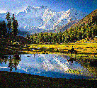
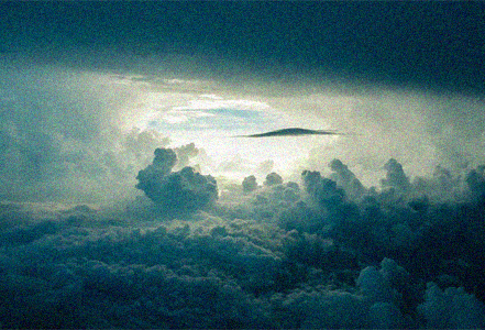
Images captured in low-light situations tend to be noisy, and lack sharp edge resolution. A common solution to this problem is to use a flash. However, while the flash image does have sharp edge definition, it suffers from an unpleasing direct-lighting effect.

We started off with the problem of filtering an image to remove noise while maintaining sharp detail in the edges. We saw how the bilateral filter solves this problem by combining two different sources of information: the weights of the filter were determined by color proximity, in addition to spatial proximity. The cross bilateral filter took the idea of drawing on multiple sources of information a step further. The RGB values for the filter came from two altogether different photos of the same scene.
In fact, this idea recurs throughout the field of computational photography. An imaging problem is solved by drawing on information from different representations, and even modalities. Together, the combined sources make up for their individual shortcomings, and provide a more comprehensive (or perhaps simply a more beautiful) picture of the world.
Please upload your Python code, input/result images, and any notes of interest as a PDF to Gradescope. Please use writeup.tex for your submission.
Bilateral filters are useful for so many image processing applications. Sylvain Paris has a gentle introduction to the topic and its many applications here.
This lab was developed by Numair Khan and the 1290 course staff. Numair created the logos and drew Sir Cameralot, with inspiration from Hergé and Tintin. Thanks to Sylvain Paris for the parameter grid example.