
Seamless image blending using gradient-domain fusion (Pérez, et al.).
Project: Poisson Image Editing
Logistics
- Files: Github Classroom.
- Extra disk space: /course/cs1290_students
- Part 1: Code
- Writeup template: In the zip: writeup/
- Hand-in process: Gradescope. Upload your repo directly to Gradescope. There is an option to import a repo on submission.
- If this fails: required files are in code/, writeup/writeup.pdf - use the
createSubmissionZip.py script.
- Submit anonymous materials please!
- Due: Weds 28th Oct. 2020, 9pm.
Background
We will explore gradient-domain image processing: a simple technique applicable to blending, tone-mapping, and
non-photorealistic rendering. In this project, we will use gradient-domain blending for seamless image compositing; so-called Poisson blending (pwa-sohn; French for 'fish'), because in the process of compositing we will solve a kind of second-order partial differential equation commonly known as Poisson's equation (after Siméon Denis Poisson).
The simplest method of compositing would be to replace pixels in a target image with pixels from a source image. Unfortunately, this will create noticeable seams even if the backgrounds are similar. How can we get rid of these intensity difference seams?
The insight is that humans are perceptually sensitive to gradients rather than absolute image intensities. Thus, we set up the problem as one of finding values for the output pixels that maximally preserve the gradients in the source region without changing any of the target pixels. Note that we
are making a deliberate decision here to ignore the overall intensity of the source region—we reintegrate (modified) source gradients and forget the absolute source intensity.
Requirements / Rubric
- +70 pts: Implement gradient-domain image blending.
- +10 pts: Test it on the six provided cases and at least one composite of your own which demonstrates a failure case of the algorithm.
- +20 pts: Write up your project (writeup/writeup.pdf), showing both input images, naive blending (directly copying the pixels as the stencil code does), and gradient-domain blending. Explain why the failure case occurs. Describe your process and algorithm, show your results as images and output values, describe any extra credit and show its effect, tell us any other information you feel is relevant, and cite your sources. We provide you with a LaTeX template in
writeup/writeup.tex. Please compile it into a PDF and submit it along with your code. In class, we will present the project results for interesting cases.
We conduct anonymous TA grading, so please don't include your name or ID in your writeup or code.
- +10 pts: Extra credit (see below)
- -5*n pts: Lose 5 points for every time (after the first) you do not follow the instructions for the hand in format
Running the stencil code is done through main.py. See the help message by running main.py -h to learn about what flags can be used to change program behavior.
Image sets are read in from a single directory. Each image to perform blending on must come with a source, mask, and target image with the correct filename format. Additionally, the directory must contain a .csv file named offsets.csv. This file is where the x and y offset values are defined for each image in the directory. If a directory of images is built with incorrect formatting, the stencil code should produce relevant error messages. Use the given data/ folder in the stencil as reference.
Potentially useful functions: We supply fix_images() in utils.py to automatically resize and move all images for easy compositing. The stencil code is set up to do this immediately. This project will make use of the scipy.sparse Python package. See the comments in student.py for more information on this.
Forbidden functions: Any pre-built Poisson equation solver (e.g., functions from the PDE module in SymPy).
Extra Credit
You are free to complete any extra credit you imagine. Here are some suggestions:
- up to 5 pts: Mixing gradients to allow transparent images or images with holes. Instead of trying to adhere to the gradients of the source image, at each masked pixel use the largest gradient available in either the source or target. You can also try taking the average of gradients in the source and target.
- up to 10 pts: Color2Gray: Sometimes, in converting a color image to grayscale (e.g., when printing to a laser printer), we lose the important contrast information, making the image difficult to understand. For example, compare the color version of the image on right with its grayscale version produced by
rgb2gray().
Can you do better than rgb2gray? Gradient-domain processing provides one avenue: create a gray image that has similar intensity to the rgb2gray output but has similar contrast to the original RGB image. This is an example of a tone-mapping problem, which is conceptually similar to that of converting HDR images to RGB displays. To get credit for this, show the grayscale image that you produce (the numbers should be easily readable).
Hint: Try converting the image to HSV space and looking at the gradients in each channel. Then, approach it as a mixed gradients problem where you also want to preserve the grayscale intensity.

- up to 5 pts: Automatically shifting the offset of the source image to decrease the difference of the images in the composite area.
- up to 10 pts depending on the method: Implement and compare other blending techniques (note: fewer extra credit points for comparing Laplacian pyramid blending as implementation was in Lab 4).
- up to 10 pts: Perform the blending on video frames instead of still images. How can we make the blending temporally consistent?
- up to 10 pts: Try other applications of gradient domain editing such as non-photorealistic rendering, edge enhancement, and texture transfer. See the Poisson Image Editing and Gradient Shop papers for some suggestions.
For all extra credit, be sure to demonstrate in your write up cases where your extra credit has improved image quality or computation speed.
Hand in
You will lose points if you do not follow instructions. Every time after the first that you do not follow instructions, you will lose 5 points. The folder you hand in must contain the following:
- code/ - directory containing all your code for this assignment
- writeup/writeup.pdf - your report as a PDF file generated with Latex.
Use Gradescope to submit your repo directly. When creating a subission, you will be asked to upload your repo. In this project, you should be able to commit images to the repo and submit through Gradescope. Make sure only the necessary images for your handin are included.
Implementation Details
Simple 1D Examples
Let's start with a simple case where instead of copying in new gradients we only want to fill in a missing region of an image and keep the gradients as smooth (close to zero) as possible. To simplify things further, let's start with a one dimensional signal instead of a two dimensional image. The example below is contained in the walkthough.py script with the starter code.
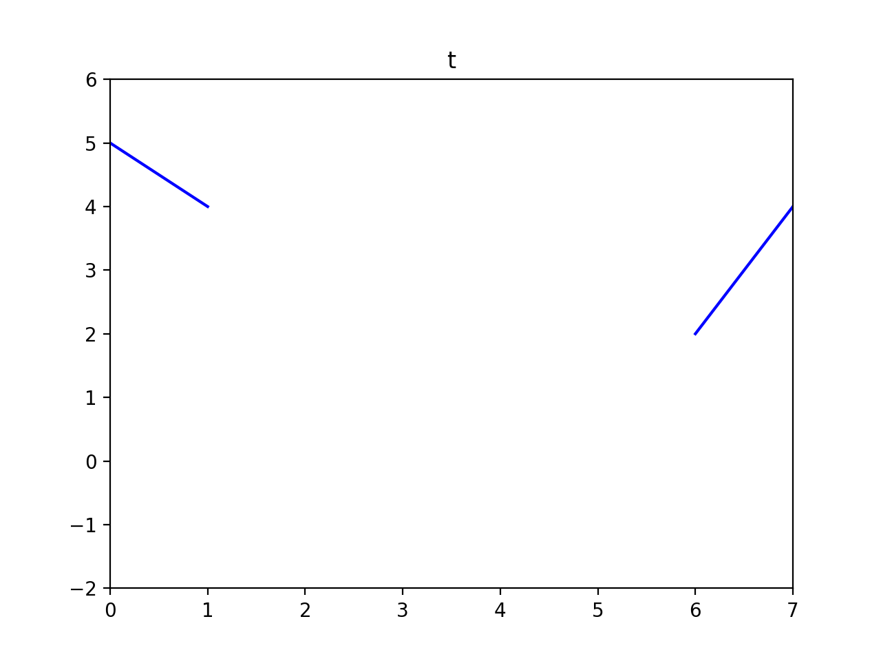
Here is our signal \(t\) and a mask \(M\) specifying which "pixels" are missing.
t = np.array([5, 4, 0, 0, 0, 0, 2, 4])
M = np.array([0, 0, 1, 1, 1, 1, 0, 0], dtype=np.bool)
We can formulate our objective as a least squares problem. Given the intensity values of \(t\), we want to solve for new intensity values \(v^*\) under the mask \(M\) such that:
$$v^*=\underset{v}{\mathrm{argmin}} \sum_{i\in M} \sum_{j\in N_i \cap M} (v_i-v_j)^2 + \sum_{i\in M} \sum_{j\in N_i \cap \sim M} (v_i-t_j)^2$$
Here \(i\) is a coordinate (1D or 2D) for each pixel under mask \(M\). Each \(j\) is a neighbor of \(i\). Each summation guides the gradient (the local pixel differences) in all directions to be close to 0. In the first summation, the gradient is between two unknown pixels, and the second summation handles the border situation where one pixel is unknown and one pixel is known (outside the mask \(M\)). Minimizing this equation could be called a Poisson fill.
For this example, let's define `neighborhood' to be the pixel to your left. In principle, we could define neighborhood to be all surrounding pixels; in 2D, we would at least need to consider vertical and horizontal neighbors. The least squares solution to the following system of equations satisfies the formula above.
Note that the coordinates don't directly correspond between \(v\) and \(t\)—the first unknown pixel \(v(0)\) sits on top of \(t(2)\). We could formulate it differently if we chose.
v[0] - t[1] = 0 # left border - note, v[0] is at the location of t=2
v[1] - v[0] = 0 # v[0] is at location t=2, v[1] at t=3
v[2] - v[1] = 0 # v[1] is at location t=3, v[2] at t=4
v[3] - v[2] = 0 # v[2] is at location t=4, v[3] at t=5
t[6] - v[3] = 0 # right border - note, v[3] is at the location of t=5
Plugging in known values of \(t\) we receive:
v[0] -    4 = 0
v[1] - v[0] = 0
v[2] - v[1] = 0
v[3] - v[2] = 0
   2 - v[3] = 0
Now let's convert this to matrix form and have NumPy solve it:
A = [[  1,  0,  0,  0 ],
     [ -1,  1,  0,  0 ],
     [  0, -1,  1,  0 ],
     [  0,  0, -1,  1 ],
     [  0,  0,  0, -1 ]]

b = [[  4 ],
     [  0 ],
     [  0 ],
     [  0 ],
     [ -2 ]]

A = np.array(A)
b = np.array(b)

v = np.linalg.lstsq(A, b, rcond=None)[0]

t_smoothed = np.zeros_like(t, dtype=np.float32)
t_smoothed[~M] = t[~M]
t_smoothed[M] = v.flatten()

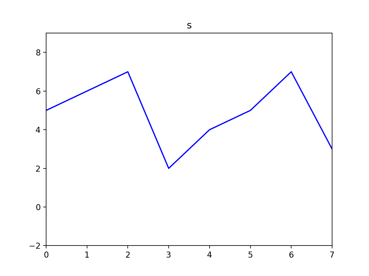
As it turns out, in the 1D case, the Poisson fill is simply a linear interpolation between the boundary values. But, in 2D, the Poisson fill exhibits more complexity. Now instead of just filling, let's try to seamlessly blend content from one 1D signal into another. We'll fill the missing values in \(t\) using the corresponding values in \(s\):
s = np.array([5, 6, 7, 2, 4, 5, 7, 3])
Now our objective changes—instead of trying to minimize the gradients, we want the gradients to match another set of gradients (those in \(s\)). We can write this as follows:
$$v=\underset{v}{\mathrm{argmin}} \sum_{i\in M} \sum_{j\in N_i \cap M} ((v_i-v_j)-(s_i-s_j))^2 + \sum_{i\in M} \sum_{j\in N_i \cap \sim M} ((v_i-t_j)-(s_i-s_j))^2$$
We minimize this by finding the least squares solution to this system of equations:
v[0] - t[1] = s[2] - s[1]
v[1] - v[0] = s[3] - s[2]
v[2] - v[1] = s[4] - s[3]
v[3] - v[2] = s[5] - s[4]
t[6] - v[3] = s[6] - s[5]
After plugging in known values from \(t\) and \(s\), this becomes:
v[0] -    4 =  1
v[1] - v[0] = -5
v[2] - v[1] =  2
v[3] - v[2] =  1
   2 - v[3] =  2
Finally, in matrix form for NumPy:
A = [[  1,  0,  0,  0 ],
     [ -1,  1,  0,  0 ],
     [  0, -1,  1,  0 ],
     [  0,  0, -1,  1 ],
     [  0,  0,  0, -1 ]]

b = [[  5 ],
     [ -5 ],
     [  2 ],
     [  1 ],
     [  0 ]]

A = np.array(A)
b = np.array(b)

v = np.linalg.lstsq(A, b, rcond=None)[0]

t_and_s_blended = np.zeros_like(t, dtype=np.float32)
t_and_s_blended[~M] = t[~M]
t_and_s_blended[M] = v.flatten()

Notice that in our quest to preserve gradients without regard for intensity we might have gone too far—our signal now has negative values. The same thing can happen in the image domain, so you'll want to watch for that and at the very least clamp values back to the valid range.
When working with images, the basic idea is the same as above, except that each pixel has at least two neighbors (left and top) and possibly four neighbors. Either formulation will work.
For example, in a 2D image using a 4-connected neighborhood, our equations above imply that for a single pixel in \(v\), at coordinate \((i,j)\) which is fully under the mask you would have the following equations:
v[i,j] - v[i-1, j] = s[i,j] - s[i-1, j]
v[i,j] - v[i+1, j] = s[i,j] - s[i+1, j]
v[i,j] - v[i, j-1] = s[i,j] - s[i, j-1]
v[i,j] - v[i, j+1] = s[i,j] - s[i, j+1]
In this case we have many equations for each unknown. It may be simpler to combine these equations such that there is one equation for each pixel, as this can make the mapping between rows in your matrix \(A\) and pixels in your images easier. Adding the four equations above we get:
4*v[i,j] - v[i-1, j] - v[i+1, j] - v[i, j-1] - v[i, j+1] = 4*s[i,j] - s[i-1, j] - s[i+1, j] - s[i, j-1] - s[i, j+1]
Where everything on the right hand side is known. This formulation is similar to Equation 8 in Pérez, et al. You can read more of that paper for guidance, especially the section on the "Discrete Poisson Solver".
Note that these formulations are not equivalent. The more verbose formulation is a constraint on first derivatives, while combining the equations effectively gives you a constraint on the discrete Laplacian. You are free to implement either approach. The discrete Laplacian method which uses one equation per pixel leads to a simpler implemention because the A matrix will be more easily indexed.
Tips
- For color images, process each color channel independently (hint: matrix \(A\) won't change, so don't go through the computational expense of rebuilding it for each color channel).
- The linear system of equations (and thus the matrix \(A\)) becomes enormous. But \(A\) is also very sparse because each equation only relates a pixel to some number of its immediate neighbors. Use SciPy's support for sparse matrices! See comments in
student.py for more information about this.
- \(A\) needs at least as many rows and columns as there are pixels in the masked region (or more, depending on how you've set up your system of equations. You may have several equations for each pixel, or you may have equations for already known pixels just for implementation convenience). If
the mask covers 100,000 pixels, this implies a matrix with at least 100,000,000,000 entries. Don't try that. Instead, use SciPy to build sparse matrices for which all undefined elements are assumed to be \(0\). There are several sparse matrix storage options in
scipy.sparse. Make sure you're using the correct option for what you need to achieve (again, see the comments in student.py to learn more about this).
- You'll need to keep track of the relationship between coordinates in matrix \(A\) and image coordinates. It would be a good idea to write a helper function that converts 2D image coordinates to their corresponding 1D index, and another function for the inverse transformation. You might need a dedicated data structure to keep track of the mapping between rows and columns of \(A\) and pixels in \(s\) and
\(t\).
- Not every pixel has left, right, top, and bottom neighbors. Handling these boundary conditions might get slightly messy. You can start by assuming that all masked pixels have 4 neighbors (this is intentionally true of the first 5 test cases), but the 6th test case will break this assumption.
- Your algorithm can be made significantly faster by finding all the \(A\) matrix values and coordinates ahead of time and then constructing the sparse matrix in one operation.
scipy.sparse matrices offer various instantiation options, including the ability to provide the data and corresponding coordinates at once. See the documentation for scipy.sparse.csr_matrix for example.
- By avoiding for loops entirely you can get the run time down to about one second, but don't worry about this unless everything else is working.
- Please read the code comments in
student.py for more suggestions.
Acknowledgements
Project derived by James Hays from Pérez et al., Poisson Image Editing, 2003. Original project specification by Pat Doran. Project revised in using material from Derek Hoiem and Ronit Slyper. Conversion from MATLAB to Python by Isa Milefchik.