
Project 2: Image Blending
Seamless image blending using gradient domain fusion
(Pérez, et al.).
Due Date: 11:59pm on Friday, September 28th, 2012
Brief
- This handout: /course/cs129/asgn/proj2/handout/
- Stencil code: /course/cs129/asgn/proj2/stencil/
- Data: /course/cs129/asgn/proj2/data/
- Handin: cs129_handin proj2
- Required files: README, code/, html/, html/index.html
MATLAB stencil code is available in /course/cs129/asgn/proj2/stencil/. You're free to do this project in whatever language you want, but the TAs are only offering support in MATLAB. One file supplied is fiximages.m which automatically resizes and moves all the images so that one could easily composite them. The stencil code is set up to do this immediately. Feel free to use or ignore this function. Another file getmask.m will allow you to interactively make an image mask.
Requirements
You are required to implement gradient domain image blending as well and to create at least one composite of your own in addition to the 6 provided test cases. Constructing your own example will help give you an understanding of the shortcomings of this algorithm.
Overview
This project explores gradient-domain processing, a simple technique with a broad set of applications including blending, tone-mapping, and non-photorealistic rendering. This specific project explores seamless image compositing via "Poisson blending".
The primary goal of this assignment is to seamlessly blend an object or texture from a source image into a target image. The simplest method would be to just copy and paste the pixels from one image directly into the other (and this is eactly what the starter code does). Unfortunately, this will create very noticeable seams, even if the backgrounds are similar. How can we get rid of these seams without doing too much perceptual damage to the source region?
The insight is that people are more sensitive to gradients than absolute image intensities. So we can set up the problem as finding values for the output pixels that maximally preserve the gradient of the source region without changing any of the background pixels. Note that we are making a deliberate decision here to ignore the overall intensity! We will add an object into an image by reintegrating from (modified) gradients and forgetting whatever absolute intensity it started at.
Simple 1d Examples
 Let's start with a simple case where instead of copying in new gradients we only want to fill in a missing region of an image and keep the gradients as smooth (close to zero) as possible. To simplify things further, let's start with a one dimensional signal instead of a two dimensional image. The example below is contained in the walkthough.m script with the starter code.
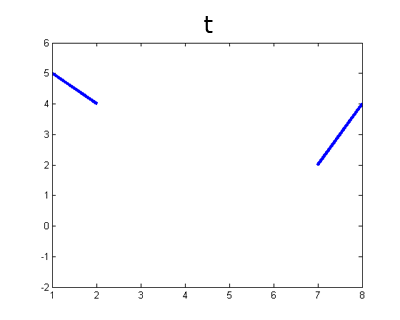
Here is our signal t and a mask M specifying which "pixels" are missing.
We can formulate our objective as a least squares problem. Given the intensity values of t, we want to solve for new intensity values v under the mask M such thatt = [5 4 0 0 0 0 2 4]; M = [0 0 1 1 1 1 0 0]; M = logical(M);
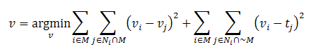
Here i is a coordinate (1d or 2d) for each pixel under mask M. Each j is a neighbor of i. Each summation guides the gradient (the local pixel differences) in all directions to be close to 0. In the first summation, the gradient is between two unknown pixels, and the second summation handles the border situation where one pixel is unknown and one pixel is known (outside the mask M). Minimizing this equation could be called a Poisson fill.
For this example let's define neighborhood to be the pixel to your left (you could define neighborhood to be all surrounding pixels. In 2d, you would at least need to consider vertical and horizontal neighbors). The least squares solution to the following system of equations satisfies the formula above.
Note that the coordinates don't directly correspond between v and t — v(1), the first unknown pixel, sits on top of t(3). You could formulate it differently if you choose. Plugging in known values of t we getv(1) - t(2) = 0; %left border v(2) - v(1) = 0; v(3) - v(2) = 0; v(4) - v(3) = 0; t(7) - v(4) = 0; %right border
Now let's convert this to matrix form and have Matlab solve it for usv(1) - 4 = 0; v(2) - v(1) = 0; v(3) - v(2) = 0; v(4) - v(3) = 0; 2 - v(4) = 0;
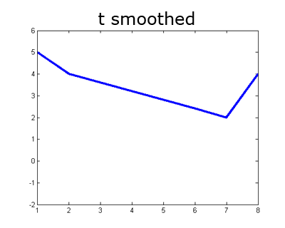
As it turns out, in the 1d case, the Poisson fill is simply a linear interpolation between the boundary values. But in 2d the Poisson fill exhibits more complexity. Now instead of just doing a fill, let's try to seamlessly blend content from one 1d signal into another. We'll fill the missing values in t using the correspondig values in s:A = [ 1 0 0 0; ... -1 1 0 0; ... 0 -1 1 0; ... 0 0 -1 1; ... 0 0 0 -1]; b = [4; 0; 0; 0; -2]; v = A\b; % "help mldivide" describes the '\' operator. t_smoothed = zeros(size(t)); t_smoothed(~M) = t(~M); t_smoothed( M) = v;
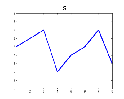
Now our objective changes — instead of trying to minimize the gradients, we want the gradients to match another set of gradients (those in s). We can write this as follows:s = [8 6 7 2 4 5 7 8];
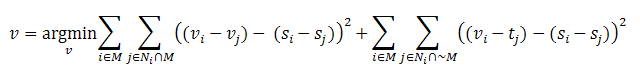
 We minimize this by finding the least squares solution to this system of equations:
After plugging in known values from t and s this becomes:v(1) - t(2) = s(3) - s(2); v(2) - v(1) = s(4) - s(3); v(3) - v(2) = s(5) - s(4); v(4) - v(3) = s(6) - s(5); t(7) - v(4) = s(7) - s(6);
Finally, in matrix form for Matlabv(1) - 4 = 1; v(2) - v(1) = -5; v(3) - v(2) = 2; v(4) - v(3) = 1; 2 - v(4) = 2;
Notice that in our quest to preserve gradients without regard for intensity we might have gone too far — our signal now has negative values. The same thing can happen in the image domain, so you'll want to watch for that and at the very least clamp values back to the valid range. When working with images, the basic idea is the same as above, except that each pixel has at least two neighbors (left and top) and possibly four neighbors. Either formulation will work.A = [ 1 0 0 0; ...
-1 1 0 0; ... 0 -1 1 0; ... 0 0 -1 1; ... 0 0 0 -1]; b = [5; -5; 2; 1; 0]; v = A\b; t_and_s_blended = zeros(size(t)); t_and_s_blended(~M) = t(~M); t_and_s_blended( M) = v;
For example, in a 2d image using a 4-connected neighborhood, our equations above imply that for a single pixel in v, at coordinate (i,j) which is fully under the mask you would have the following equations:
In this case we have many equations for each unknown. It may be simpler to combine these equations such that there is one equation for each pixel, as this can make the mapping between rows in your matrix A and pixels in your images easier. Adding the four equations above we get:v(i,j) - v(i-1, j) = s(i,j) - s(i-1, j) v(i,j) - v(i+1, j) = s(i,j) - s(i+1, j) v(i,j) - v(i, j-1) = s(i,j) - s(i, j-1) v(i,j) - v(i, j+1) = s(i,j) - s(i, j+1)
Where everything on the right hand side is known. This formulation is similar to equation 8 in Pérez, et al. You can read more of that paper, especially the "Discrete Poisson Solver", if you want more guidance.4*v(i,j) - v(i-1, j) - v(i+1, j) - v(i, j-1) - v(i, j+1) = 4*s(i,j) - s(i-1, j) - s(i+1, j) - s(i, j-1) - s(i, j+1)
Note that these formulations are not equivalent. The more verbose formulation is a constraint on first derivatives, while combining the equations effectively gives you a constraint on the discrete Laplacian. You are free to implement either approach, discrete Laplacian method which uses one equation per pixel leads to a simply implemention because the A matrix will be more easily indexed.
Implementation Tips
- For color images, process each color channel independently (hint: matrix A won't change, so don't go through the computational expense of rebuilding it for each color channel).
- The linear system of equations (and thus the matrix A) becomes enormous. But A is also very sparse because each equation only relates a pixel to some number of its immediate neighbors.
- A needs at least as many rows and columns as there are pixels in the masked region (or more, depending on how you've set up your system of equations. You may have several equations for each pixel, or you may have equations for already known pixels just for implementation convenience). If the mask covers 100,000 pixels, this implies a matrix with at least 100,000,000,000 entries. Don't try that. Instead, use the sparse command in Matlab to build sparse matrices for which all undefined elements are assumed to be 0. A naive implementation will run slowly because indexing into a sparse matrix requires traversing a linked list. If you're building the sparse A matrix in a for loop it will take 5 to 30 seconds. Test your algorithm on smaller images first.
- You'll need to keep track of the relationship between coordinates in matrix A and image coordinates. sub2ind and ind2sub might be helpful (although they are slow, so you might want to do the transformation yourself). You might need a dedicated data structure to keep track of the mapping between rows and columns of A and pixels in s and t.
- Not every pixel has left, right, top, and bottom neighbors. Handling these boundary conditions might get slightly messy. You can start by assuming that all masked pixels have 4 neighbors (this is intentionally true of the first 5 test cases), but the 6th test case will break this assumption.
- Your algorithm can be made significantly faster by finding all the A matrix values and coordinates ahead of time and then constructing the sparse matrix in one operation. See sparse(i,j,s,m,n,nzmax). This should speed up blending from minutes to seconds.
- By avoiding for loops entirely you can get the run time down to about one second, but don't worry about this unless everything else is working.
- Helpful matlab commands that may help you speed up your algorithm: sparse, speye, find, sort, diff, cat, and spy.
- imblend.m in the starter code contains some more suggestions.
- The TAs are fully aware of the implementations available on the internet, we'll know if you used them.
Write up
For this project, just like all other projects, you must do a project report in HTML. In the report you will describe your algorithm and any decisions you made to write your algorithm a particular way. Then you will show and discuss the results of your algorithm. Also discuss any extra credit you did. Feel free to add any other information you feel is relevant.
For all results, you should show both input images, as well as the naively blended version (directly copying the pixels as the stencil code does), and then finally your version.
You should show some failure cases (which shouldn't be too hard to find) and conjecture about why they didn't work.
Extra Credit
You are free to do whatever extra credit you can think of. Here are some suggestions:
- Mixing Gradients to allow transparent images or images with holes. Instead of trying to adhere to the gradients of the source image, at each masked pixel use the largest gradient available in either the source or target. You can also try taking the average of gradients in the source and target.
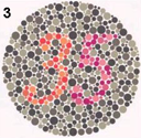
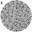
- Color2Gray: Sometimes, in converting a color image to grayscale (e.g., when printing to a laser printer), we lose the important contrast information,
making the image difficult to understand. For example, compare the color version of the image on right with its grayscale version produced by rgb2gray().
Can you do better than rgb2gray? Gradient-domain processing provides one avenue: create a gray image that has similar intensity to the rgb2gray output
but has similar contrast to the original RGB image. This is an example of a tone-mapping problem, conceptually similar to that of converting HDR
images to RGB displays. To get credit for this, show the grayscale image that you produce (the numbers should be easily readable).
Hint: Try converting the image to HSV space and looking at the gradients in each channel. Then, approach it as a mixed gradients problem where you also want to preserve the grayscale intensity.
- Automatically shifting the offset of the source image to decrease the difference of the images in the composite area.
- Implement and compare other blending techniques, such as Laplacian pyramid blending.
- Perform the blending on video frames instead of still images.
- Try other applications of gradient domain editing such as non-photorealistic rendering, edge enhancement, and texture transfer. See the Poisson Image Editing and Gradient Shop papers for some suggestions.
Graduate Credit
To get graduate credit on this project you must do one form of extra credit of sufficient difficulty. Any one of the suggested extra credit satisfies this requirement.
Handing in
This is very important as you will lose points if you do not follow instructions. Every time after the first that you do not follow instructions, you will lose 5 points. The folder you hand in must contain the following:
- README - text file containing anything about the project that you want to tell the TAs
- code/ - directory containing all your code for this assignment
- html/ - directory containing all your html report for this assignment (including images)
- html/index.html - home page for your results
Then run: cs129_handin proj2
If it is not in your path, you can run it directly: /course/cs129/bin/cs129_handin proj2
Rubric
- +70 pts: Seamless image blending implementation
- +10 pts: At least one composite you constructed on your own
- +20 pts: Write up
- +15 pts: Extra credit (up to fifteen points)
- -5*n pts: Lose 5 points for every time (after the first) you do not follow the instructions for the hand in format
Credits
Project derived from Poisson Image Editing by James Hays. Original project specification by Pat Doran. Project revised in using material from Derek Hoiem and Ronit Slyper.