Background

For my final project, I wanted to supplement some of the work our group did on the panorama stitching project using the Nokia N900 phone. I abandoned the phone, replacing it with my handy point-and-shoot Canon Powershot SD960 IS. In order to view the panoramas with full rotation about the camera's position, I tapped the Google Maps API, which lets developers create their own panoramas using its Street View controls.

My original goal was to detect motion between several 360° panoramas and connect them in Street View using the relative positions and camera orientations. I did not succeed in doing this. See the Bundler section for details. Spherical projection and Laplacian blending were also added to improve upon our original project.

Process

Implementing 360° panoramas proved to be more time-consuming than I had expected. The entire pipeline had to be rewritten to get wrapping from the last image to the first image to line up properly. When images are stitched together, the relative Y-axis position of the images varies slightly between images. When stitching 10-12 photos together, this vertical drift can accumulate to be very significant. The total drift needs to be calculated before compositing the images and distributed between all the images in order for the first and last images to vertically align. Our original pipeline loaded two images at once, projected them into cylindrical coordinates, computed the features, found the matches, computed the homographies, composited the images, and then repeated for the next pair of images. For this project, I had to perform each step for all images at once. This resulted in a major rewrite. I saved and loaded temporary images as necessary to avoid keeping all input images in memory at once. Each step of the process is described below.

Computing the Field of View

In order to project an image in cylindrical coordinates, we need to know the camera's horizontal field of view. This value is useful to know before taking photos as it can help provide an estimate of how many pictures are needed to complete a full 360° of rotation. For spherical projection, we need the camera's vertical field of view. Both values were calculated by taking a photo of a sheet of graph paper with the paper encompassing the entire horizontal or vertical dimension, depending on which value we were calculating. Knowing the size of each square (0.25 inches) and the distance of the camera from the paper, I was able to come up with an estimate for each value. I took both pictures with camera in its lowest zoom setting.

Since a rotation of the camera is simply a translation in cylindrical/spherical coordinates, RANSAC is used to find only x and y translations to align the images. This eliminates the need to compute a homography and solve a system of equations. Finding the homography, however, can help us determine whether the field of view is correct. Using a pair of images to be stitched, I found the homography using several different field of view angles. I calculated the mean of the element-wise error from the identity matrix and selected the angle that minimized this error. I found the horizontal field of view first, projecting the image in cylindrical coordinates. For spherical coordinates, I fixed the horizontal FOV at the optimal value I found in the previous step and performed the same calculation on the vertical FOV.

The horizontal field of view was calculated at 66.5° and was found to be approximately 59.5°. The vertical field of view is smaller, as expected, at 53.1°. Its true value was not far off, at 52.6°.

Cylindrical/Spherical Projection

Cylindrical and spherical projection requires knowing the camera's field of view in 1 and 2 dimensions respectively. While this is a little bit of an overhead, it produces better looking panoramas (as seen in our project 6 results) and simplifies the math in other steps of the process by eliminating the need to find a homography. Projecting the image coordinates into cylindrical and spherical coordinates is a little tricky though.

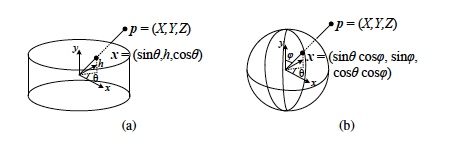
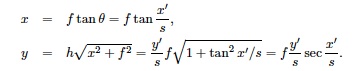
Knowing the horizontal field of view, we can determine θ based on the image's x coordinate. θ's value changes from -FOV/2 to FOV/2 as x moves from 0 to width-1. I mapped the coordinates of the image in cylindrical coordinates to a coordinate system ranging from -1 to 1 on both the u and v axes and used the inverse mapping equations to find the appropriate point from the original image for each pixel in the resulting image.

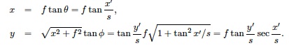
Since the Street View API takes in spherical panorama projections for viewing, I was hoping to do at least 1 vertical stitch. The problem comes down to knowing the value φ, which is the vertical camera tilt angle. There were some major issues that were preventing me from performing panoramas of vertical stitching in addition to horizontal stitching.

• Lining up horizontal photos was somewhat challenging even with a tripod. Vertical stitching was much harder. I tried two approaches for vertical images: taking a full row of pictures and then returning to the original position and tilting the camera up, and tilting the camera up and down before turning it clockwise to line up the next horizontal photo. Both approaches resulted in drastic vertical drift, even with the help of the tripod's level for calibration.
• φ was difficult, if not impossible, to measure correctly. I may have been able to determine it after finding my translations. Cylindrical projections are always the same regardless of how the camera is tilted. With spherical projections, the image becomes more compressed as the pixels get closer to the sphere's poles, where there are major discontinuities. Panorama stitching apps on camera phones work well since they can use the phone's accelerometers or gyroscope to calculate φ, making vertical stitching in spherical coordinates much simpler.
• Google Maps has one of these to capture its photos. I didn't.

Finding Image Translation

SURF features and ratio matching are used for feature matches. RANSAC is run with 4000 iterations to find a pair of points used to determine a translation. As previously mentioned, we don't need to find 4 points or solve for a homography when only finding translation. It was much easier for images to be properly aligned when removing scaling and rotation. In project 6, we often found that homographies for certain images were wildly inaccurate, even for images that had a large number of feature matches.

Calculating Vertical Drift

After calculating the translations between each pair of images, I find the translation between the last image and the first image. With the all the translations, we can determine the absolute y position of the first image at each end of the image. These two images must line up vertically. The difference between the two positions is divided by the number of total images in the panorama and each image is skewed by this value to fix this alignment. Images end up being shifted no more than 3 pixels from their original translations, though this can make poor alignments noticeably worse.

Compositing Images

Images are aligned based on the translation values in relation to the previously composited image. Relative translations are converted into absolute positions so we know exactly where to composite each image and how to maintain the proper image dimensions. The region where the two images overlap is blended using Laplacian blending. Results could have been improved using Poisson blending and graph cuts. As OpenCV and C++ are not suited for solving large systems of equations very easily, I steered clear of this route after some initial exploration.

One of the challenges of 360° panoramas is getting the transition from the end to the beginning to look seamless. In order to do this, I stitched the first image to the last image and cropped everything after the blended region. This way I can avoid very visible seams from 359° to 0°. This worked for all but 1 of my images.

Bundler

It was a little ambitious of me to think I would be able to do 360° panoramas and determine structure from motion for several panoramas. Thankfully, Noah Snavely has released a toolkit for performing Structure from Motion from unordered image collections called Bundler. I thought this would save me time and meet my main goal. Installing Bundler turned out to be a time sink as there were undocumented configuration issues. Once I had it set up, I could not find camera positions for more than 2 images (my demo required just 3) no matter how many images or what combinations of images I tried. With only 2 values, I was not able to make sense of the values (rotation matrix and translation vector) in a way that could be translated into data for Google Maps.

Bundler is an extremely powerful library, as evidenced by Snavely's own Photo Tourism work with Richard Szeliski and Steven Seitz and by other examples on the web. It just didn't work for my cases, though I only tried a few test cases besides my panoramas. My time may have been better spent developing my own crude method based on feature matching.

Using Street View

The Street View API is fairly easy to use if you have at least some familiarity with JavaScript. I had to pad my images to have a 2:1 width-to-height ratio in order for them to display properly. In my testing, I found that results look strikingly different in different browsers. I tested with Firefox 4 on a Mac, Google Chrome 12 beta on a Mac, and Chrome 10 & 11 for Linux. On Linux, the curved tops of cylindrical and spherical projections appear straight. This is from Google Maps and nothing I did. It was strange to see different behaviors in the same browser on different operating systems.

Results

View 360° Results

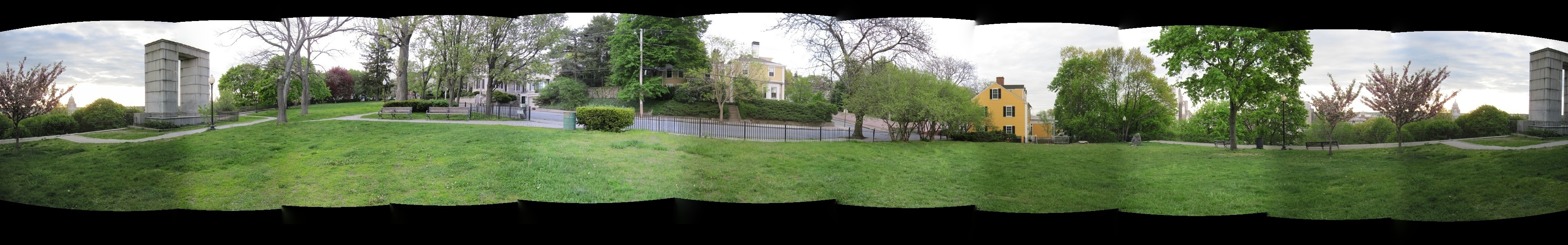
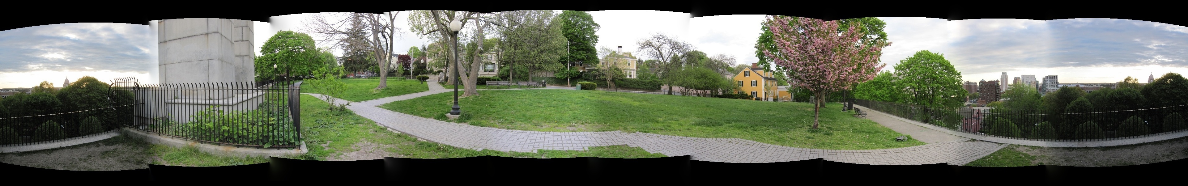
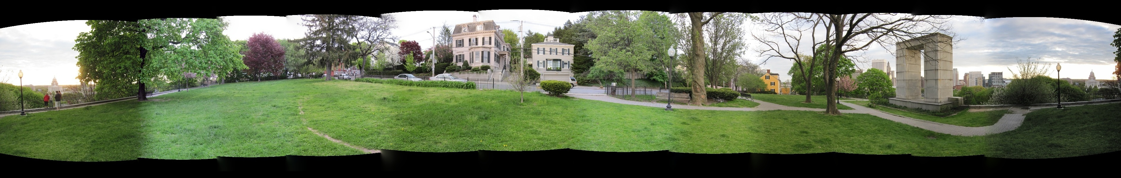
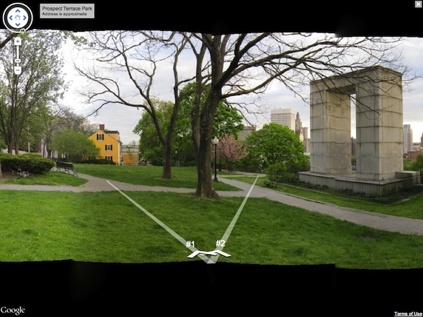
I took 3 panoramas, a total of 33 images, at Prospect Terrace Park at sunset as I was starting on my code. This proved to be a good decision as it was one of the last night days we had for the next week and a half. Lighting differences can be seen between images in the panoramas. Some photos were taken with the camera facing directly into the setting sun. In others, you can tell that the lighting changed gradually between the time of the first picture to the last (takes about 2-3 minutes to adjust the tripod and take all the pictures).

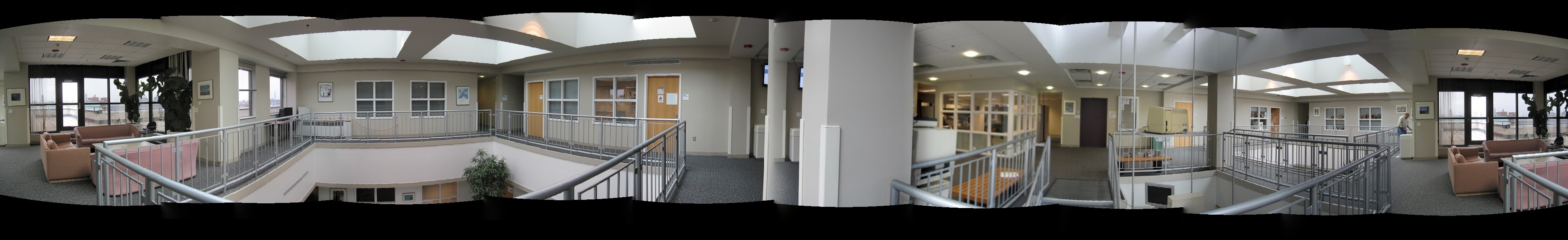
I also took one panorama from the top floor of the CIT. There are some issues with alignment and focus in the image containing a pillar close to the camera.

The demo has controls at the bottom for toggling between alpha blended and Laplacian blended source images. Alpha blending left strange artifacts at the tops of images where the photos did not overlap but the alpha value was less than 1.0. It also produced blurriness where photos did not line up perfectly.

Laplacian blending is a major improvement. Between images that are accurately vertically aligned and have similiar lighting conditions, the seam is almost invisible. In other cases, the blending only serves to make varying lighting and poor alignments less jarring. Black is blended into the tops and bottoms of images that have significant vertical drift. This is still an improvement over the artifacts and blurriness introduced by alpha blending.

Below are regular panoramas (no compensating for vertical drift). These can serve as comparison to the panoramas in Street View.

(Click a picture to view. Navigate through images using left/right arrow keys)