Activity 1-3

1. Make a copy of ACT1-3 and save it to the your Google Drive. Open it and go to the OffsetExample sheet.
2. Change the contents of cell B10 and notice that cells A11 and B11 automatically update to display the average of the homework number you specify. Verify that it works for a number of homeworks.
3. Look at the formula in cell B11. This is a combination of two functions, AVERAGE and OFFSET.

   First, notice how the functions are "nested" within each other (you are getting the average of the output of another function).

   Next, examine how the OFFSET function refers to cell B10 - 1. The value of the expression B10 - 1 is how many “steps” to the right to take from the starting cells (B2:B7) to get to the homework you're interested in.

   For example, if B10 is 9, then (B2:B7) is offset by 0 cells down and B10 - 1, or 8, cells to the right. This gets us all the scores for HW9, which is what we want as input for the AVERAGE function. Make sure you understand how this works before moving on.

4. Now suppose we want to enter a name in B13 (such as “Barry”) and then see the student's average for all homeworks in cell B15. First off, you need to determine what row is Barry's row. Write a formula (using the MATCH function) in cell B14 that identifies the row of the student whose name is in B13. Check that your formula works on several students' names.
5. The formula for cell B15 is similar to the formula in cell B11. Copy the formula in cell B11 into cell B15. Modify it to find the average of the student mentioned in cell B13. Remember that we found the student's row number for a reason.
6. What happens when you mistype a name in B13? To avoid the problem, we can have the user select a name from a list of possibilities. Go to the Data tab and select "Validation". Under criteria, click the grid icon and use the mouse to select the student names. Next, select List from a range and specify a data range of names that we want. Finally, save the validation. This option is listed under “Data Validation” because it verifies what kind of data can be put in the cell.

1. Open the spreadsheet you finished in ACT1-2. You should have three sheets: PivotTable, RawData, and SandersCompare.
2. Copy the sheet GeneralCompareTemplate from ACT1-3 to your spreadsheet. Right-click on the sheet and click Copy to... and select the current spreadsheet. Rename it GeneralCompare.
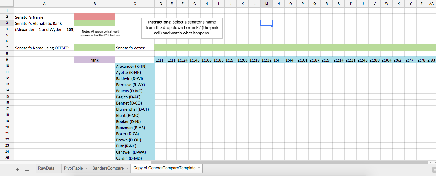
3. New Rule: We want to reference as many cells as possible (using functions). This helps you (and us!) understand where everything is coming from. Use functions (like =PivotTable!A5) to fill the row and column headers (starting in the blue boxes). You should fill to the box that has 'num_agree' in it, which will be around Row 114; your last senator should be Wyden. Your spreadsheet should now look something like this (click to see it bigger):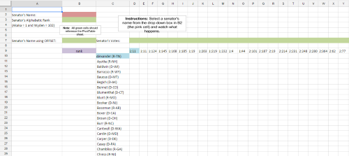
   
4. Use Data Validation to allow a list of names in cell B2. These names can be referenced from the same sheet (C10:C114).
5. In cell B3, use the MATCH function to get the senator's alphabetic rank. Reference cells from PivotTable because other sheets might be sorted differently. In this rank, we want Alexander to be 1 and Wyden to be 105.
6. In cell B7, use the OFFSET function to display the senator's name. You should offset a cell from the PivotTable sheet (which should be sorted alphabetically). The number of rows to offset should be based on the alphabetic rank we just computed.
7. In cells D7:AL7, modify the function in B7 to display the senator's votes. How many rows should you offset? How many columns? You will need to use an absolute reference ($) to make sure you always use cell B3.
8. We can now fill the table. Copy the function from cell SandersCompare!B2 to cell D10 and modify it. Remember that the row we want to compare to is in row 7 on this sheet.
9. Use the COUNTIF function to again compute num_agree, num_disagree, and num_not_voting in columns AB:AD (the orange cells).
10. Finally, compute the rank of each senator in column B (purple cell) by using the formula $$\frac{\text{num_agree}-\text{num_disagree}}{\text{num_agree}+\text{num_disagree}}$$
11. For this sheet, we won't sort by decreasing order (there is a way to do dynamic sorting - you can Google it). Select Sanders from the list and verify by eye that some of the ranks are the same on GeneralCompare and SandersCompare.

We're done with this activity. Keep a few things in mind:

1. We didn't have to have the green cells in this sheet. We could have entered a very large and complicated function in cell D10. But doing it step-by-step is a good idea because (1) it breaks the large problem into manageable pieces and (2) it will be easier to figure out what we did later.
2. Nice formatting with cells and text boxes also help with understanding and readability.
3. This is an interactive spreadsheet - people can mess with it and make their own conclusions about the data.