Introduction to Statistical Estimation

This tutorial is also used as an excuse to introduce and discuss somewhat the notion of a neural representation.
 
 

1. Random Variables

X is called a random variable (r.v.), it can take only two values, and we write:

P(X = 1) = p; P(X = 0) = 1-p

Note that the probability of each outcome is a non-negative number, and the sum of these numbers over all possible outcomes is equal to 1.

This simple model captures our uncertainty about the neuron's state before we observe it. Observing the neuron's state is an experiment, whose outcome is the r.v. X.

If we performed the experiment 1000 times under the exact same conditions, we would expect about 1000 x p of the outcomes to be 1.

Also, p is the mean (or expectation) of the distribution, denoted E(X), i.e., the sum of all possible values of X weighted by their respective probabilities:

E(X) = 0 x P(X = 0) + 1 x P(X = 1) = 0 x (1-p) + 1 x p = p

2. Point Estimation

p* = P(X = 1) = (1/N) _i  X_i

Quite generally, this is what statistical estimation is all about:
 

Such an estimator *  is called a point estimator in statistics textbooks because it concerns a single parameter of the distribution. Later, we shall discuss more complicated examples of estimation.

How good an estimate is *? In other words how close is it to the true value  ? Remember that * is derived from a collection of realizations of the random variable X. Therefore * is itself a r.v., and it has a certain probability distribution.

In our case, where   is p, the mean of the distribution, it can be shown that * converges to   when N goes to infinity. This means (among other things) that the mean square error (MSE) of the estimator, E( | * -  | ) goes to 0 when N goes to infinity. This is (roughly) the law of large numbers.

In general, an estimator *  which converges to the true value   of the target parameter when the size of the dataset converges to infinity is called a consistent estimator. Evidently, consistency is a highly desirable property.
 

3. Joint Probabilities

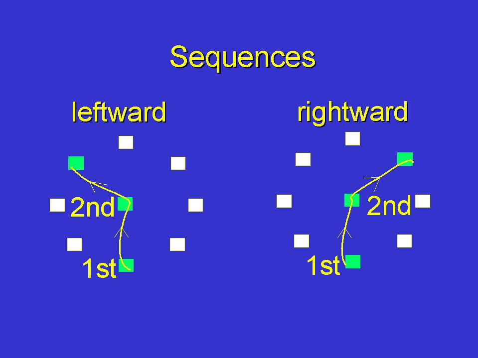
For the moment, we consider a simpler task, with only one segment: the monkey is instructed to move its arm from the central position to one of the eight targets that may appear on the screen. Let Y denote the actual movement direction. Then Y can take 8 values:  Y = 0, Y =  / 4,  Y =  / 2, Y = 3 / 4, ...

Again Y is a r.v.:  before we observe it, we are uncertain about its value.

Denote by Z the cue on the computer screen. Z  is a r.v. which can take the same 8 values. We assume that they all occur with equal probability P(Z = z) = 1/8.

If the monkey performed the task with 100% accuracy, we would have Y = Z. Unfortunately, even the best of monkeys make mistakes. As a result, the relationship between Y and Z can be less than trivial.

To capture this relationship, we use a joint probability distribution on the two random variables Y and Z. Such a joint probability distribution has to specify the probabilities of each of the 64 possible values of the pair (Y,Z). These 64 probabilities are non-negative numbers which must add up to 1.
 
 
 

4. Conditional Probabilities

There often is. Suppose the monkey is performing correctly 90% of the time and when he's wrong the direction he chooses is uniformly distributed over the 7 wrong values. We can then use conditional probabilities to define the model rather painlessly.

First, we say P(Z = z) = 1/8 = .125 for all z.

Then we say that the conditional probability that Y = z  given that  Z = z  is .9, and for any y  z the conditional probability that Y = y  given that  Z = z  is .1/7.

The conditional probability that Y = y given that  Z = z is denoted P(Y = y | Z = z) (sometimes simply P(y | z) if it's clear from context which random variables go in which position).

So we have P(Y = z | Z = z) = .9, and, for y  z , P(Y = y | Z = z) = .1/7  .0143.

Now, how often does the outcome (Y = y and Z = z) happen? Well, Z = z happens 12.5% of the time, and of all the outcomes such that Z = z  the fraction with Y = z is 90%. Therefore, the total probability  P(Z = z and Y = z) is .125 x .9 = .1125

Similarly, for y  z, P(Z = z and Y = y) = .125 x .0143  .00179.

The model has thus been completely specified.

The mathematical property of conditional probabilities that we just used is:

P(Y = y and Z = z) = P(Z = z) P(Y = y | Z = z).

This can actually be taken as a definition of the conditional probability. This is intuitive: of all outcomes such that Z = z, the fraction that yields Y = y is the ratio  P(Y = y and Z = z) / P(Z = z).

5. Independent Random Variables

In that case, only 16 outcomes (Z,Y) have positive probabilities. As before, P(Z = z) = 1/8 for all z.
So we get P(Y =  / 2 and Z = z) = P(Z = z) P(Y =  / 2 | Z = z) = (1/8)x(2/3) = 1/12.
Similarly, P(Y = 3 / 2 and Z = z) = P(Z = z) P(Y = 3 / 2 | Z = z) = (1/8)x(1/3) = 1/24.

Again the model has been completely defined using conditional probabilites.

Note that here P(Y = y | Z = z) does not depend on z at all. Therefore, P(Y = y) = P(Y = y | Z = z).

This property of the joint variables Y and Z, P(Y) = P(Y | Z),  is called statistical independence. In words, marginals and conditionals are the same.

(NOTE: P(Y=y) is called the marginal probability of y because when P(Y and Z) is displayed in a 2-D array with Y varying say along the columns, it is customary to write P(Y = y), the sum of the entries of the Y=y row, in the margin.)

Equivalently, Y and Z are independent if P(Z = z) = P(Z = z | Y = y): since the monkey does not pay attention to the stimulus, we shouldn't pay attention to the monkey if we want to find out what the stimulus was.

Also, by the definition of a conditional probability, independence is equivalent to P(Y and Z) = P(Y)P(Z):

Two random variables are independent if their joint probability is the product of their marginals.

6. Bayes rule

Thanks to this trick, the monkey has now realized that there are eight directions, and we shall assume that half of the time he moves his arm in the correct direction z, whatever that is.

Suppose we observe the arm movement direction Y and we want to know what Z was. Certainly we should pay attention to Y now, since the monkey paid attention to Z: the two rv's are not independent any more.

Since Z is a r.v., the most complete answer we can hope for is the conditional P(Z | Y). This is called the posterior probability of Z, because it follows the observation Y. In contrast, the marginal P(Z) is called the prior probability of Z.
 
But the model specified only the conditionals P(Y | Z). This is natural, because there is a clear causal relationship from stimulus to movement direction.

How do we go backward and compute the conditional P(Z | Y), i.e. the posterior?

First, we use the definition of the conditional: P(Z | Y) = P(Y and Z) / P(Y). Then, we substitute P(Y | Z)P(Z) for P(Y and Z), and we get:

P(Z | Y) = P(Y | Z)P(Z) / P(Y).

This is called Bayes formula.

We're almost done. We know P(Z), because it's the prior. We know P(Y | Z), because it was given in the model (monkey is  correct half of the time).
The last ingredient is P(Y), which is not given in the model, but can be computed easily: we "decompose" the event Y = y into all the outcomes (Y,Z) such that Y = y, and we sum all the probabilities of these outcomes:

P(Y = y) = _i P(Y = y and Z = z_i) = _i P(Y = y | Z = z_i) P(Z = z_i)

so that Bayes formula finally reads

P(Z = z | Y = y) = P(Y = y | Z = z) P(Z = z)  /  _i P(Y = y | Z = z_i) P(Z = z_i).

All the quantities appearing in this formula are known, so we can now compute the posterior  P(Z | Y).

7. The Neural Representation of Movement Direction

As before, let the random variable X denote the neural activity. Using the electrode array shown above, X can be a multi-dimensional random variable describing the activity of more than one neuron.

The physiologist observes X and ask questions about Y (or, more ambitiously, about Y and  Z). This allows him/her to investigate various models of how the brain works: such models are incomplete at best, and the physiologist wants to submit them to various tests.

Neurons in motor cortex, even the large neurons in primary motor cortex that send an axon down the spinal cord, don't directly control muscle  activity. So the picture is roughly that there is a special circuitry, partly in cortex partly in other structures, which reads out the state of the brain and transforms it into a suitable pattern of motoneuron firing (motoneurons are the cells in the spinal cord that directly control muscle contractions).

That "state of the brain," to be read out and transformed into a specific movement,  must contain all the parameters of the movement, including its direction. So, calling that state X, we see that the transformation we are talking about amounts to computing Y given X.

Note that the probability P(Y | X) had better be very peaked around its mean, in order for the movement to be accurate.

The neurophysiologist, who wants to test his/her model about brain function, mimicks the computation performed by the brain, by predicting the movement direction from the observed cortical activity. If the prediction is good, i.e., matches the actual direction, the model of neural representation of movement direction entertained by the neurophysiologist is deemed satisfactory.

To state things a bit more carefully, showing that a given model allows one to get a good prediction P(Y | X) indicates that the model is not inconsistent with brain performance.

The model that the neurophysiologist is testing in this way contains a number of ingredients, to be discussed now.

8. Conditional Expectation (Regression)

The physiologist's model computes P(Y | X) using Bayes formula: P(Y | X) = P(X | Y) P(Y)/P(X). (It then uses this to derive a value y for any given observation X=x. For instance, one can use the most likely direction y, defined as the y that maximizes the function p(y) = P(Y = y | X = x). Or, the mean E(Y | X = x) can be used.)

An essential ingredient of this model is the quantity P(X | Y = y), which characterizes the firing of the cell for different movement directions y.

In this tutorial we shall focus on E(X | Y = y), the mean value of P(X | Y = y), i.e., the conditional expectation of X given Y. In statistical textbooks, this conditional expectation is also called the regression of r.v. X on r.v. Y.

Note that the regression, which is a bona fide deterministic function of y, is completely determined by the two jointly random variables X and Y. As such it  is almost always:

The last point deserves to be mentioned because "regression" is sometimes understood to mean "linear regression."  Yet if X and Y are two joint r.v.'s which describe a given phenomenon, say in biology, physics or economics, chances are that the relationship between y and the conditional mean of X given that Y = y is not linear.

Since the regression function is unknown, it is in general estimated from observed pairs (X_i,Y_i). In some cases of course, we may wish to use a linear model for our estimate of the regression function. This will be the case if we have reason  to believe that the true regression function is approximately linear.

Here, the regression is called the tuning curve of the neuron (for movement direction) and is denoted f(y) = E(X | Y = y).

(If we want to use Bayes' formula in a mathematically correct way, we should derive the whole distribution P(X | Y = y) rather than just its mean tc(y). This is a rather ambitious task, but it can be done.)

In what follows, we shall use the following terminology, inspired from psychology:

9. Estimating a Regression Function

Estimating this f(y) is not fundamentally different from point estimation, as examined in Section 2 of this tutorial. It is just a bit more complicated, because:

The question then is how to make the best possible use of this limited dataset D, i.e., get estimates for f(y) that have the least possible MSE.

Note now that from an MC ("mathematically correct") perspective, this criterion makes sense only with respect to an underlying joint distribution for (Y,X). Since no such underlying distribution is known, we use a heuristic criterion. This consists, essentially, in assessing the quality of our estimator when used to predict the actual movement, as outlined above.

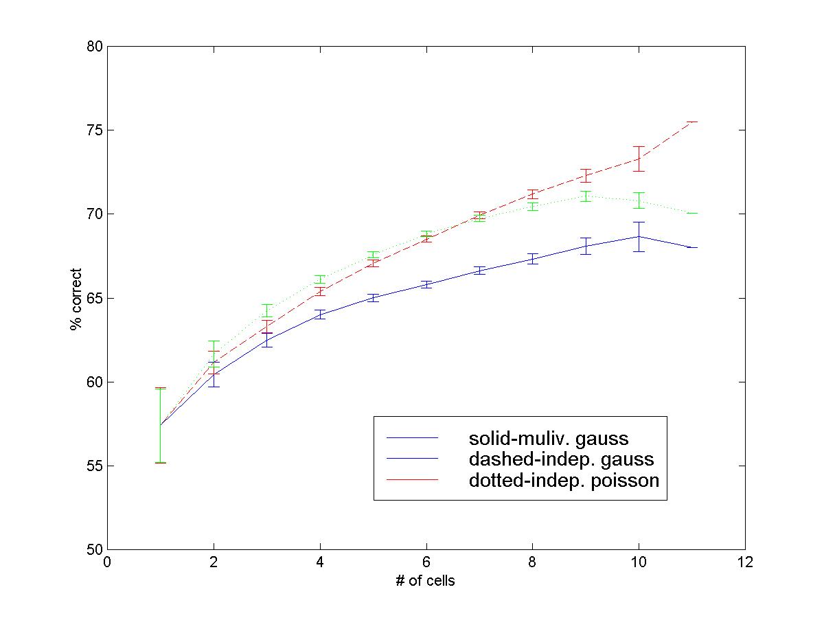
For instance, the following figure (courtesy of Nicho Hatsopoulos) compares the outcomes of three different predictions for the second segment in a sequential task, resulting from using three different models for estimating P(X | Y). The observed firing in this case is a multidimensional spike count, representing the activity of from 1 to 11 neurons, as indicated on the x-axis of the figure.

This activity is recorded before movement onset, i.e., before the first segment is performed. The prediction however concerns the direction of the second segment. The details of this study, e.g. the fact that the entire distribution P(X | Y), rather than just the regression E(X | Y) is estimated (under various suitable parametric forms), are not critical for the present discussion. What is important is that the physiologist uses the quality of the prediction P(Y | X) afforded by various estimators P(X | Y) ) to make a statement about the goodness of these estimators, hence, indirectly, about the nature of the neural representation of movement direction. In this case, what is at issue is the representation of the second segment in a sequential task, and this requires the use of a carefully designed regression model.
 
 
 

To illustrate some issues arising in the estimation of a regression function, we shall now use a simulated example, meant to reproduce the simple experiment outlined in sections 7 and 8.

In this example, Y is movement direction and X is a 1-dimensional spike count (single neuron). We create, artificially, a "true" tuning curve x = f(y), and our goal will be to estimate the value of the tuning curve at 8 regularly spaced points on the circle. The estimator will use a dataset consisting of 50 observed pairs (X_i,Y_i).

The tuning curve we use in this example is a triangle-shaped function, which reaches its maximum for y = .
Observations are made at 50  randomly placed points  Y_i  in the interval  [0,2]. For each such Y_i, we observe X_i
= Y_i  +  noise_i  , where  (noise_i),  i = 1,... 50,  are 50 independent random variables of mean 0.
 

In the figure, the fifty observations (X_i,Y_i) are represented as blue triangles pointing upward. The black circles are the 8 target values: (0 , f(0)) , ( / 4 , f( / 4)) , ( / 2 , f( / 2)) , (3 / 4 , f(3 / 4)) ,... These target values lie on the "true" triangular-shaped tuning curve x = f(y), which is unknown (for the purpose of this problem).
 
 

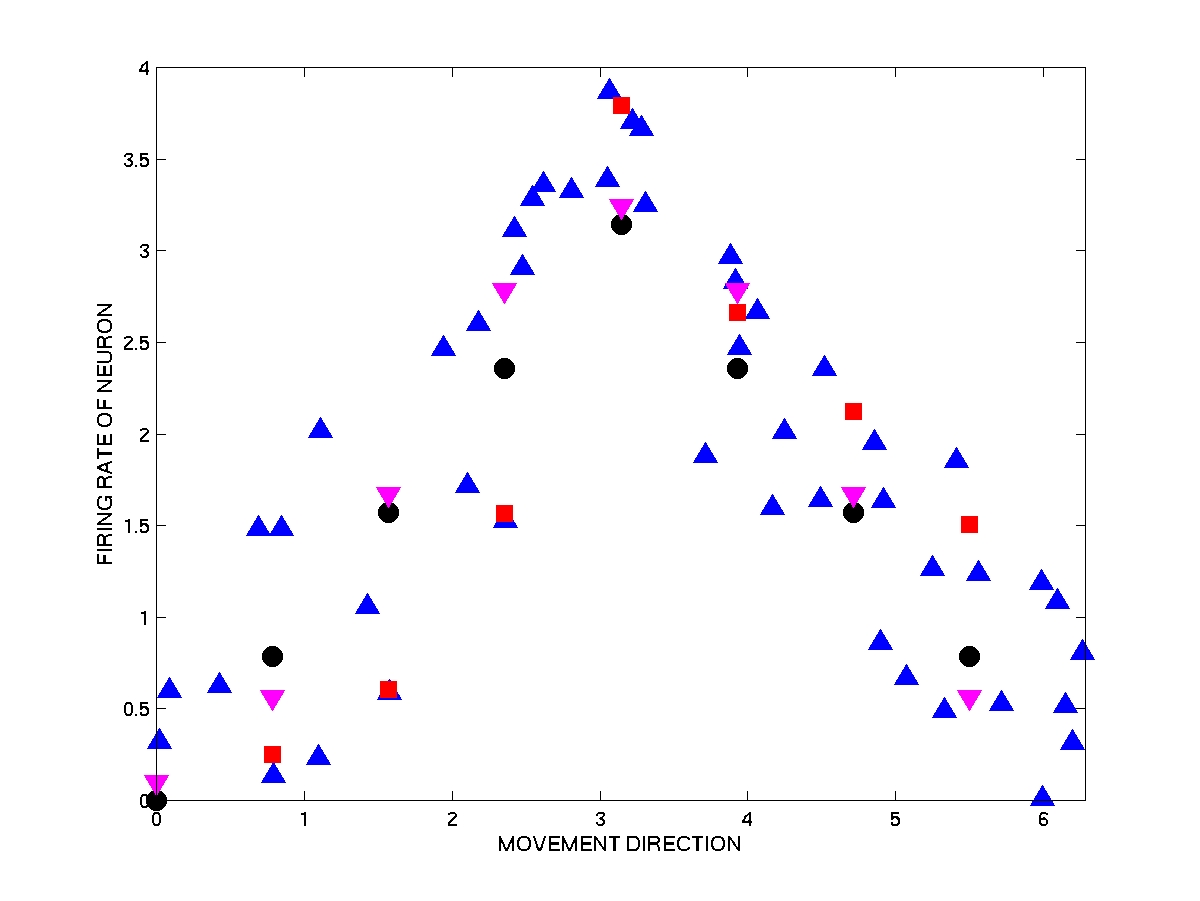
Consider first the estimator given by linear interpolation, i.e., by drawing line segments between adjacent data points. Let's denote this estimator by f*(y) (remember that f* is random, since it depends on the observations). The 8 values of f* at the 8 points of interest are represented in the figure by red squares.
 
 

10. Variance of Estimator

In short, our estimate f* suffers from high variablility. Now the amount of variability of a random variable X is conveniently measured by its variance, the mean square deviation of X from its mean E(X). Formally: Variance(X) = E [ (X-E(X)) ].

Cortical neurons usually have a fairly large variance:  two identical trials will yield very different spike counts X. Therefore, if we had another realization of the dataset, we would most likely get a very different X_i for each Y_i (assuming that we sample the same directions Y_i). This variance of  the dataset is reflected directly in the variance of the estimate f*(y).

Another way to characterize this flaw of f* is to say that this estimator overfits the data: linear interpolation pays too much attention to individual sample points, as it tries to accommodate each one  of them individually. This is a poor strategy to use, because these data points are known to be intrinsically unreliable.
 

11. Bias of Estimator

This can be done in a variety of ways, more or less appropriate for any given problem. A quite popular smoothing strategy to use for direction tuning curves of motor cortical neurons is to fit the data with a cosine function. This estimator, which we denote f**, is a smooth function which is known to approximate rather well the tuning curves of motor cortical neurons.

Thus, we now impose a certain functional form on our estimator, and the problem  boils down to adjusting a small number of  parameters, in this case the offset, the phase and the amplitude of the function. Typically, the parameters are adjusted to minimize the sum of square distances between the observed data points and the regression (just like in linear regression).

In the figure above, the 8 estimates  f**(y_i)  are represented as purple triangles pointing downward. Note that they provide a much better approximation to the "true" tuning curve than the first, highly variable, estimator f*. The reason is that, thanks to the parametric form of f**, all observations now contribute to the estimate at any given point y, as opposed to just the two nearest observations in f*. This results in a drastic reduction of variance, hence a better estimate.
 
Is it the case that the more smoothing the better? Certainly not. Consider the smoothest of all possible approximations to the dataset, a constant function f***(y) = (1/N) _i X_i . Note that by taking the average of the N observations we reduced the variance of our estimator as much as we possibly could. On the other hand, by oversmoothing in this way,  we completely removed the dependency of the estimator on the independent variable y, which of course results in a very poor estimator.

Another way to describe what is happening here is to say that we introduced too large a bias in our estimator f***. Bias refers to a systematic difference between the estimate and the true f(y), one that does not go away when the sample size goes to infinity. In fact the bias is the difference between the expected value of the estimate (remember that the estimate is a random variable since it depends on the data D) and the true f(y).

12. Bias/Variance Dilemma

It is a relatively straightforward calculation to prove the following theorem: The mean square error of any estimator is MSE = Bias + Variance. Thus, in the best of worlds we would like to have both Bias and Variance equal to 0.

We saw however, in the two extreme examples f* and f***, that this could not be achieved. In effect, it turns that, quite generally, reducing variance cannot be done without introducing bias, and vice-versa.. The optimal strategy is then highly problem-dependent: we want to introduce some bias, to reduce the excess of variance, but not too much bias.

Even more important is the type of bias to use. As discussed above, smoothness is a sensible all-purpose form of bias. There are however better types of bias for specific applications. Thus, in the case of direction tuning curves, a good type of bias, based on specific knowledge about the properties of cortical cells, consists of using a parametric model in the shape of a cosine function. We saw that the resulting estimator, f**, yielded much better results than either the high-variance f* or the high-bias f***.

Note that the very particular form of bias imposed by f** would result in a high MSE, i.e., poor performance, if the true f(y) was very different from a cosine function, for instance if it was bimodal rather than unimodal. However, since most cells in primary motor cortex have a unimodal tuning curve for movement direction, the cosine model allows one to reduce the variance without introducing too much bias, thereby achieving a reasonable compromise.
 
 

13. The ``Curse of Dimensionality''

If a regression model is completely general,
i.e.,, if it is not specifically designed to fit a narrowly defined class
of joint random variables, it will, in general, behave poorly.

Consider the case studied above, where the independent variable, Y, is movement direction. This r.v. is one-dimensional, and it is therefore rather easy to achieve good performance. In fact all of the discussion above is really just fine tuning: any bias-introducing method that assumes some smoothing but not too much smoothing will do the job, provided a large enough dataset D is used. Moreover, "large enough" in this case is by no means unreasonable.

Contrast this situation with a problem of estimating a regression function on a high-dimensional independent variable.

Consider for instance the extremely active domain of object recognition in computer vision. Roughly, the independent variable, Y, is an image of an object (possibly within a natural scene), and the dependent variable, X, takes its value in a collection of labels, say chair, table, computer printer, ice skate, etc.

From the fact that our brains are so good at assigning the correct label to an object occurring in a natural visual scene, it is apparent that the true regression function is extremely peaked: when an object is present in a scene, there is hardly any ambiguity at all as for its label. However, the problem of unconstrained object recognition in computer vision is still, by and large, unsolved.

Although the difficulty in cracking this problem can be analyzed in other ways, the statistical-estimation framework may offer an interesting perspective. Suppose we wanted to estimate the regression function from a dataset of image-label pairs, where images are taken from general, unconstrained, natural scenes.. We would of course fail, and this failure may be tracked to the fact that the image to be analyzed--the independent variable--is extremely high-dimensional. Therefore, a dataset D that would do a good enough job at covering the regions of interest in Y-space would have to be, essentially, of astronomical size. Fine-tuning smoothing methods would be of little help here.

Note that one class of statistical estimators that have been extensively used in an attempt to solve object-recognition problems consists of so-called artificial neural networks. In these models, estimation is often called learning, the independent r.v. is often called the input, and the dependent r.v. is often called the output. The parameter   to be adjusted in an artificial neural network is a very high-dimensional vector of  parameters, often called synaptic weights. This high dimensionality guarantees that the model is very general: it can accommodate, theoretically, virtually any regression function. (Such estimators are called non-parametric is statistical textbooks, precisely because the dimensionality of their parameter space is so high that these models are completely general. In contrast, a parametric estimator is one with a low dimensional parameter space, e.g. the cosine-function model for direction tuning discussed above.)
 

14. Structured Representations and Compositionality

A natural conclusion is therefore that brains probably rely on the use of a specific sort of bias, particularly apt at modeling natural objects and scenes.

From the poor level of performance of today's computer vision (as compared to natural vision), it is probably safe to conclude that the nature of this bias still largely eludes us. However, one may speculate that this bias has to do with the compositional nature of the objects occurring in natural scenes.

In brief, compositionality refers to our ability to construct structured mental representations, hierarchically, in terms of parts and their relations. The rules of composition are such that:

It may be, however, that context-free grammars are too narrowly defined, or perhaps simply inappropriate, to allow useful learning, in the form of parameter estimation, for natural problems, whether in linguistics or in vision. Developing more appropriate forms of compostitional models thus appears to be one of the main challenges for future research in these fields.

In parallel to these modeling efforts, one will need to understand how structured compositional representations are implemented in neural activity. One hypothesis that has received much attention in recent years is that the mechanism whereby brains compose neural representations with each other uses the fine temporal structure of the spiking processes of interconnected neurons. In the notation introduced in the preceding sections, the r.v. X that describes the state of the brain at any given time is not a (multi-dimensional) spike count any more. Rather, it is a much more complicated stochastic object called a (multi-dimensional) point process. While this opens up tremendous possibilities for the implementation of structured representations, it also makes for much more intricate problems of statistical estimation.
 

15. Bibliography