The goal of this assignment is to implement a path planning algorithm for a SmURV robot. The SmURV is to navigate a two dimensional space, avoiding known locations with obstacles, traveling from its initial location to a goal location. Given localization information (robot pose, obstacle location, goal location), our task was to implement a path planning decision maker, and a motion control module to execute it. Specifically, the problem can be formed as follows:
The algorithm we implemented is a variant of RRT-Connect1. The goal of this write up is to show that our variant of RRT-Connect (dubbed RRT-Relax) is a good path planning algorithm due to its near optimal performance, simplicity, and efficiency. The purpose for implementing this path planner is so that it can be used in real time, allowing the SmURVs to play one on one soccer.
Path planning is an important area of robotics. Without it, a robotic agent cannot truly achieve autonomy. The ability to not only react to changes in your environment, but plan ahead in the future is an important aspect of intelligence, and therefore of great interest to roboticists. Path planning algorithms are not only of interest to roboticists. Algorithms that can efficiently traverse a search space (or subset of one) have many applications. Some other search algorithms, such as A* search and Dijkstra's, require a discretized state space, causing them to be somewhat inaccurate in continuous physical spaces. Although these algorithms are complete and optimal, their large running time is a drawback, especially when implemented for real-time path planning for autonomous robots. Potential fields is another path planning algorithm derived from the simulation of a physical system. This method, however, is prone to becoming stuck in local minima. The algorithm we used, RRT-relax, uses rapidly-exploring random trees (RRT) as the tree-based data structure by which we search our space. We chose to use RRT-relax because of it's simplicity, elegance, intuitiveness, and efficiency.
The following helper algorithms help build and maintain a rapidly exploring random tree of size K.
The method initalizeTree(q) initializes a tree data structure with q as the root. The method randomState() returns a random state (x,y value) in state space C, which is the soccer field in our implementation.
The method nearestNeighbor(q, T) returns the closest node in T to q (which is the randomly selected node in our case). The subroutine newConfig(q, qnear, qnew) incrementally checks from qnear to q to a distance e (some empirically tested constant), resulting in the new location qnew. It returns true if this new node qnew is in Cfree, and there exists an unobstructed path from qnear to qnew. It also sets the node qnew (allowing extend to manipulate it). These functions allow Extend to take in a tree, a random state, and output whether or not that random state was reached, advanced to, or trapped by an obstacle.
These two functions will create an RRT such that all nodes and edges are in Cfree.
Using these RRTs, a few more functions should be introduced before the algorithm RRT-relax.
The Connect function is a repetitive form of Extend, which continues to extend until the node qnew is equal to the node passed in, q. This is the greedy function of RRT-relax. The RelaxPath function takes a path as an input (a list of nodes), and returns a relaxed path. It does so by iterating through each node from start to end. For each node, you iterate backwards through the nodes, and if an unobstructed path exists from the current front node to the current back node, you remove the nodes in between. The pseudocode is below.
RRT-relax (as well as RRT-connect), takes in two nodes, qinit and qgoal - the starting state and the goal state. The algorithm maintains two RRTs, one with the root at the initial state, and one with the root at the goal state. At each step, one tree randomly explores a new state, while the other attempts to connect to this new state. A connection is found when the two trees find a common node. A path is returned, combining the route from the connected node to each of the two roots. This path is then relaxed - nodes that can be bypassed are removed in order to make the path more direct.
The Connect function greedily attempts to connect the two trees based on line of sight. If the connect function does not return REACHED, the trees swap behavior. This allows both nodes to randomly explore their local search space. Once the connection is established, a path is returned (from one root to the other). Then the path is relaxed. This relaxation, coupled with the greedy Connect function, is especially well suited to one on one soccer as the field has few obstacles. This allows for more direct and smoother paths toward the ball (and toward defensive positions).
Because RRT-relax is efficient, we were able to adaptively plan paths. Before Hefty traveled along any edge in the path, he checks for legality. If the path is no longer legal, he searches for a new path (from his updated position). A path is deemed illegal if the current step is obstructed, or if the goal position is altered (by the ball moving, or by an obstruction entering the goal position). Furthermore, our paths are relaxed in real time. If Hefty veers off course (due to a miscalculation in his motion controller or a late packet, he bypass any unnecessary nodes from his own location. This will also allow him to take a new path if an obstruction is removed.
Our motion controller involves two types of motion - rotation and translation. Because localization is provided (specifically the pose - x, y and r), Hefty's angle and the angle he needs in order to travel to the next node in his path can be determined. Hefty is turned toward this angle as a function of the difference in his current angle and his needed angle. Once Hefty's angle is close enough to the goal angle, he will begin to move forward, still rotating by a function of the difference in angles. This allows him to continue move forward more continuously, providing a more efficient path traversal.
When Hefty is in position to score a goal (i.e. his position, the ball's position, and the goal's position are collinear, and he is behind the ball), he attempts to push the ball forward. The goal scoring feedback control loop tells Hefty to push the ball forward. When the ball veers off to one side, he compensates by rotating proportionally to the angle created by the lines (ball, goal) and (hefty, goal). He turns toward the ball, and continues pushing forward, rotating back toward the goal. While he is pushing the ball, he starts slowly, accelerating through it. This was implemented so he doesn't push it too far in front of him. The acceleration allows him to maintain some degree of contact and control.
In order to model the state space of the game of soccer, we used a finite state machine. We broke the game into two main states:
These states are based solely on ball location - if the ball is closer to Hefty's goal (defending), he will enter the Defense state. If the ball is closer to the opponent's goal (attacking), then he will enter the Offense state.
Within these two main states are sub states (also called action states). The offensive sub states are
The defensive sub states are
Within the offense/defense state, the action states are determined by the opponent's location.
On offense, if the opponent is closer to the ball, Hefty will move into an intercepting position between his own goal and the ball (about halfway). While in this intercepting position, he will move forward toward the ball, attempting to get into a scoring position. Once he is in a scoring position, he will push the ball toward the goal, accelerating through it. If he starts out closer to the ball, he will move straight toward a scoring position, and attempt to push the ball in the goal.
On defense, if the opponent is closer to the ball, Hefty will move toward his own goal. Once he arrives in a position such that he is between his own goal and the ball, he will drive toward the ball, trying to clear it out of his zone. If he is closer to the ball than his opponent, he will bypass going to the goal, and go straight to the ball.
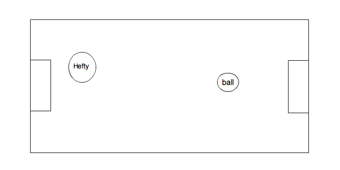
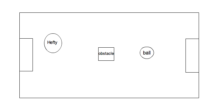
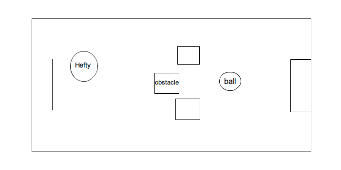
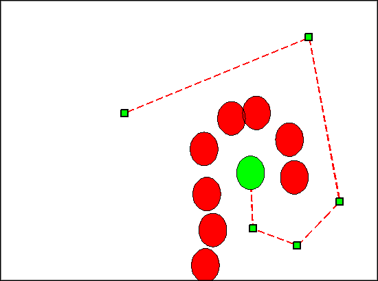
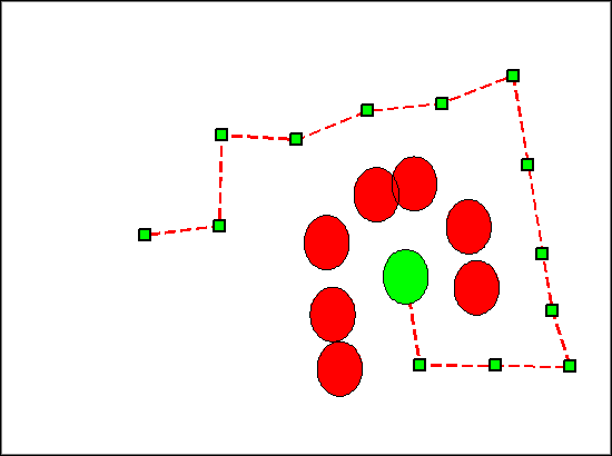
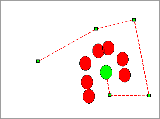
Besides the soccer competition and testing, we ran three separate timed trials. We varied the number and location of obstacles on the field. We held the start pose and the ball's location constant. We timed An example of the initial fields for each trial can be seen below.
For each of our trials we ran our client three times. Below are times for each trial, both using relaxed and unrelaxed paths. The times are from the start until a goal is made.
As you can see, relaxing the path almost cuts the time it takes for Hefty to achieve his goal in half. It is empirically observed that the relaxed path is far more optimal than the unrelaxed, random path.
The results of our soccer playing was also positive. Hefty, although slower and jerky, performed very well in the soccer competition. Our defensive strategy paid off, as he is protective of his goal. Some shortcomings, however, were noticed in his dynamic path planning and shooting ability. He is unable to approach the ball at an angle that isn't collinear with the ball and goal. This allowed him to only take one type of shot - straight toward the goal. This also forced him to clear the ball from behind, and not from the side. An improvement to this strategy will assuredly improve Hefty's soccer strategy.
The following videos show a different trial we ran with Hefty.
Unrelaxed:
Relaxed:
Unrelaxed:
Relaxed:
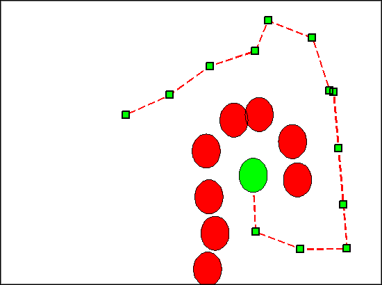
The strengths of our path planning algorithm lie in its efficiency, intuitiveness, near optimality and probabilistic completeness. Using randomly-exploring random trees as a vehicle for path planning is naturally intuitive. Planning a path in the real world can be thought of as a greedy random walk. Throughout a human traversal in an unfamiliar (and perhaps dynamic space), one may attempt random directions, averting obstacles as they move in and out of their next path. Furthermore it doesn't require a discretized state space, as both Hefty's soccer field and the real world are continuous. As displayed above, our relaxation procedure noticeably improves the path, pushing it closer to optimality.
In testing our implementation of RRT-relax, we noticed that paths were somewhat unpredictable. Furthermore, the path is usually not a smooth one. The smoothness of the path is in part determined by the e value, which determines the maximum distance between nodes in the RRT before relaxation. Furthermore, our motion controller navigates the path in a rather jerky manner. And although this algorithm is probabilistically complete, it is not complete in practice. Its level of completeness is determined by K, which limits the size of the two RRTs. With a larger space, it becomes less likely for a constant K to return a path. Furthermore because the state space is randomly searched, an optimal path is not always returned. Also, our specific implementation may not scale well in large search spaces. While checking for validity of certain locations is linear on the size of the set of obstacles, our path relaxation method is worst-case O(n2), where n is the size of its current path. As paths become larger, this time will explode.
Although our path planning implementation has a fair amount of room for improvement, RRT-Relax is an improvement over RRT-Connect, and a functional algorithm for a real-time path planer. When combined with the aformentioned soccer strategy, RRT-Relax becomes an important decision making tool for Hefty. Our motion controller is somewhat inconsistent, but this can be improved with a better feedback control system. A better feedback controller may convert the discontinuous, angled path into a smoother trajectory that the robot can follow. This would speed up the robot's performance, and would cut down on how jerky his motion is.
- Andrew Miller (amiller)