HW6: REINFORCE and REINFORCE with Baseline

Due Friday, 11/22/19 at 11:59pm

What is learning? According to the dictionary, it is "the modification of behavior through practice, training, or experience."

But, how do we learn?

In previous assignments, we have had labeled data. We could feed in an input, and tell our model to predict our labels.

However, what if we do not know what those labels are? What if we do not know much about our task either? How do we learn if we only have something that tells us how good or bad we are doing?

Introduce...reinforcement learning! Here in this assignment, we will be tackling this deep question by learning how to play Cartpole, the world's most thrilling and entertaining game, using two RL algorithms: 1) REINFORCE and 2) REINFORCE with Baseline.

Getting the stencil

You can find the files located on the "Files" column under the Assignments page. The files are compressed into a ZIP file, and to unzip the ZIP file, you can just double click on the ZIP file. There should be the files: assignment.py, reinforce.py, reinforce_with_baseline.py, and README. You can find the conceptual questions located on the "Conceptual Questions" column in the Assignments page.

Data

All data for this assignment will be collected interactively, via the CartPole-v1 environment of OpenAI Gym (woohoo!).

OpenAI Gym provides an easy to use interface for AIs to play games.

You can give the gym environment an action, and it will 1) update the state of the game, and 2) return you the next state, the reward of taking the action, and whether you arrived at a terminal state.

In CartPole you are training a simple agent (a cart) to balance a pole. Hence, CartPole.

Logistics

Work on this assignment off of the stencil code provided, but do not change the stencil except where specified. Changing the stencil will result in incompatiblity with the autograder and result in a low grade. You shouldn't change any method signatures.

For this assignment, you will need to install the OpenAI Gym library using pip install gym and matplotlib with pip install matplotlib (only if you're working locally---it's already installed in the course virtual environment).

To run the virtual environment on a department machine, you can run:

You can also check out the Python virtual environment guide to set up TensorFlow 2.0 on your local machine.

Part 1: REINFORCE

This is the first RL algorithm you will implement for this assignment. This part of the assignment will be done in reinforce.py.

The REINFORCE algorithm is a Policy Gradient method. In other words, it directly learns a function for mapping states to probability distributions over possible actions. It then samples from this distribution to pick its next move.

Going forward, "model" refers to the neural net that generates a policy and trains the policy for the agent, and the "agent" uses the policy and gathers data.

init

In the __init__ function you will be taking in two parameters: state_size and num_actions. state_size represents the number of parameters that define the state and num_actions represents the number of actions in the environment. Here you will create a feed forward network that will take an input of size [-1, state_size] and produce a probability distribution of size [-1, num_actions] (note: the [-1, num_states] shape means any 2D array where the number of columns is state_size. The -1 says the number of rows can be anything!).

Recommended Layout of the REINFORCE Feed Forward Network: 1) 1 Dense layer with outputs size hidden_size (where hidden_size is up to you) 2) 1 Dense layer with outputs size num_actions and with softmax activation

Note: The last layer must be one with outputs size num_actions and with softmax.

call

In the call function your model will take your state(s) and return your "policy" for how it should behave in those state(s). The call method will take in a batch of states with shape [episode_length, state_size] and return a policy of shape [episode_length, num_actions]. Notice here that episode_length represents the number of steps taken in the one whole episode of a game (and may vary across different episodes). The policy represents, at every time step, a probability distribution over the action space.

loss

In the loss function you will take in states, actions, and discounted_rewards. states is the history of states encountered throughout the episode, and will be of shape [episode_length, state_size]. actions is the history of actions taken in the episode, and is a list of integer indices of shape [episode_length]. discounted_rewards represents the discounted sum of future rewards for each timestep in the episode, and has shape [episode_length].

To calculate the loss you want to look at the actions you took and weight the negative log probability that you took that action by its discounted reward.

The formula for the loss our model minimizes is:

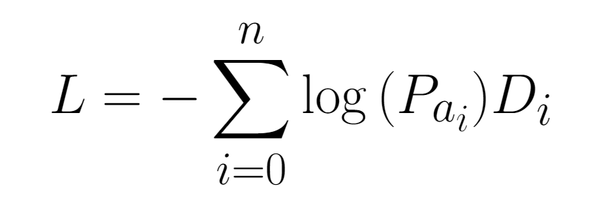
Here, $P_{a_i}$ is the probability that our agent gave the action it actually took at time $i$, which is $a_i$. $D_i$ is the discounted reward from time $i$.

To compute model.loss, we encourage you to follow these steps:

1. First, use the states in the trajectory and your model's forward pass to recompute the probability distribution over actions in the trajectory. This will be a matrix with shape [episode_length, num_actions]. You can recompute it by calling your model on the states again. This may be a bit unconventional compared with previous assignments where we passed our probabilites directly into our loss function, but this was a conscious design choice to ensure modularity. When implementing part 3, it'll become clear why we need our loss function to take in our states directly.
2. Use the action indices to gather the probabilities for actions that were selected when acting in the environment. These are our $P_{a_i}$. This will be a [episode_length] array.
3. Then take the negative log of these selected action probabilities to get an array of size [episode_length].
4. Then element-wise multiply this with discounted_rewards. If an action has a low probability and a high reward or it has a high probability and a low reward then its loss will be high.
5. Lastly return the sum of these losses.

Part 2: Training

This part will be implemented in assignment.py.

Discounted Rewards

The value of taking a given action should not just be the single reward resulting from that action. This is because the benefits of taking a "good" action could be seen later on in the episode. Instead, your estimate for the reward resulting from an action should also take account future rewards in timesteps after the agent (controlled by the model) took that action. However, sooner rewards are probably more related to our action, while rewards farther into the future are probably less dependent on that action.

Please fill out the discount function that will map our [episode_length] size rewards list containing the reward received at each time step to the discounted sum of future rewards from that time step, using the discount factor.

The formula for discounted reward is as follows:

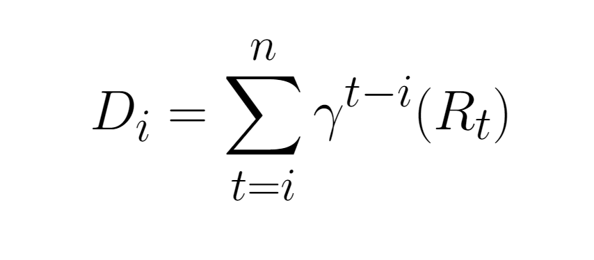
Where $D_i$ represents the discounted summed reward at time step $i$. $n$ is the number of time steps in the episode. $R_t$ is the reward at time step $t$.

One way to implement this is to iterate backwards through your rewards array $R$. At each step, you can multiply $D_{i+1}$ by $\gamma$ and add $R_i$. Recall also that $\gamma$ represents the discount factor and is usually set to 0.99.

train

Your train function will take in the environment and the model and you will train on one episode. Using tf.GradientTape, call generate_trajectory on the environment and model to get states, actions, and rewards. Convert states to a numpy array and pass them into your model's loss function, where you'll use the model's call function to get your action probabilities. Calculating your loss will require a history of the discounted rewards throughout the episode; with the discounted rewards, calculate the loss on this episode and use the tape to apply the gradients. Lastly, return the total reward of the game, which is the sum of the rewards across the episode (not discounted). If both part 1 and 2 work correctly, the model should successfully be trained on Cartpole!

Running the Model

Your assignment.py should be able to run both your RNN and Transformer model. You can run it with:

python assignment.py [MODEL TYPE]

Where MODEL TYPE is "REINFORCE" or "REINFORCE_BASELINE."

Part 3: REINFORCE with Baseline

Do not attempt part 3 without first completing and testing part 1!! Otherwise, welcome to part 3! This part of the assignment will be done in reinforce_with_baseline.py and will build directly off of part 1 (that's why it's important that part 1 works before moving on to this part).

init

In the __init__ function you will be taking in two parameters: state_size and num_actions. Again, state_size represents the number of parameters that define the state and num_actions represents the number of actions in the environment. Since REINFORCE with Baseline builds off of REINFORCE, feel free to just copy paste your network defined in part 1's __init__! Note that this is now our actor network, as it returns the "policy" which defines how the agent will act.

What spices up this algorithm, though, is that you will also need your "baseline", or "critic". This is a new separate feed forward network that will take an input of size [-1, state_size] and produce an array of values of size [-1, 1] (1 value per inputted state) that estimates how "good" that state is. Hence, we'll call this other network the critic network. Note that since the output of the critic network is values, the softmax function should not be applied.

Recommended Layout of Critic Feed Forward Network: 1) 1 Dense layer with outputs size hidden_size (where hidden_size is up to you) 2) 1 Dense layer with outputs size 1

Note: The last layer must be one with outputs size 1 and cannot use softmax.

call

In the call function you will want to call your actor network on your states which will yield your "policy" distribution across actions for each state. You again can reuse this from part 1!

value_function

In value_function, you will want to call your critic network on the batch of states, which will yield the estimated value for each state in the batch.

loss

This loss function will also be a bit more different from part 1's. As before, the loss function you will take in states, actions and discounted_rewards, which all represent the same things as in part 1.

Here we need to calculate the loss over our actor network and our critic network, which are two separate networks.

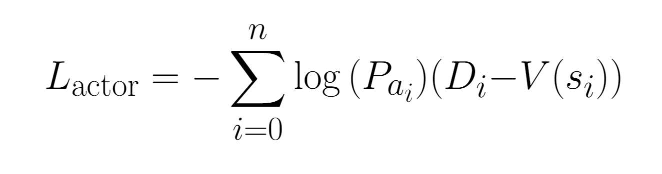
The actor loss here is almost the same as in the Reinforce Algorithm. However, there is one critical difference: We now also feed our state, $s_i$ into our critic to get $V(s_i)$, the value our critic gives the state.

$D_i - V(s_i)$ is our Advantage. It represents the difference between the discounted reward our agent earned, and how good our critic expected that state to be.

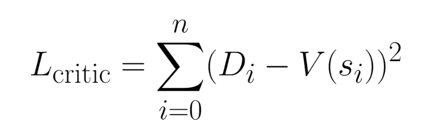
We also want to make sure our critic learns as well. Our critic loss is the squared difference between its prediction of the states value, and the discounted rewards the agent recieved from a state.

To compute this, we recommend the following:

1) To calculate the loss for your actor network you'll want to do the same thing as in part 1, with one specific change. For Step 4, instead of element-wise multiplying with discounted_rewards, you want to element-wise multiply with your advantage. Here, advantage is defined as discounted_rewards - state_values, where state_values is calculated by the critic network.

2) PLEASE TAKE NOTE OF THIS CRUCIAL STEP! In your actor loss, you must set advantage to be tf.stop_gradient(discounted_rewards - state_values). You may need to cast your (discounted_rewards - state_values) to tf.float32. tf.stop_gradient is used here to stop the loss calculated on the actor network from propagating back to the critic network.

3) Calculate the loss for your critic network by calling the value_function on the states and then taking the sum of the squared advantage.

The total loss should be equal to a weighted sum of the actor network loss and the critic network loss (we recommend the critic's loss to be weighted by 0.5).

Requirements

Our autograder will call your train function for 650 episodes to train it. After your model is trained, we will test by collecting rewards over the last 50 episodes, using your actor function to make decisions. For REINFORCE, you must receive an average reward > 200 over the last 50 episodes. For REINFORCE with baseline, you must receive an average reward > 300 over the last 50 episodes. Each model must not take over 7 minutes to train on a department machine. As a reference, our REINFORCE trains within 5 minutes and can get up to average reward of 400+, and our REINFORCE with baseline trains within 5 minutes and can get up to average reward of 450+.

Visualizing performance

We have provided the function, visualize_data, which plots the reward through episodes.

In addition, if you would like to see your agent perform, call env.render() every time you perform an action. It is useful to see how your model is learning to perform a given task. When you turn your assignment in however, turn rendering off.

README

Please submit a README were you record the performance of both architectures, and note any bugs.

Conceptual Questions

Fill out conceptual questions and submit in PDF format. Submitting a scan of written work is also fine as long as it is readable. Please copy over the questions and write well thought out answers to the questions.

CS2470 Students

Please complete the CS2470-only conceptual questions in addition to the coding assignment and the CS1470 conceptual questions. Note: Questions about 2470 will only be answered on Piazza, or by TAs marked with an asterisk (*) on the calendar.

Handing In

You should submit the assignment using this Google Form. You must be logged in with your Brown account. Your assignment.py, reinforce.py, and reinforcewithbaseline.py should be Python files, while the written up conceptual questions have to be PDFs. The README can be any format.

Acknowledgements:

This assignment is based on the REINFORCE assignemnt written by previous TAs, with edits/conversion to TF 2.0 done by:

• Kevin Du
• Daniel Ritter
• Bryce Blinn
• Naveen Srinivasan
• Brendan Le
• Zachary Horvitz
• Brian Oppenheim
• Amy Pu