
For this lab, we're going to try some real-time image processing, similar to the demos that James has shown in lecture. To begin, we need to install an additional component in MATLAB: the MATLAB Support Package for USB Webcams. Please follow the instructions here to install it.
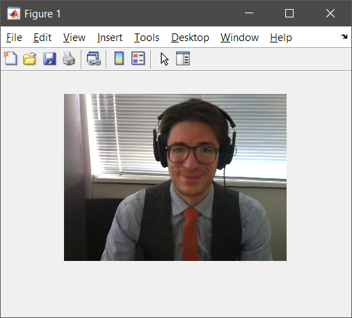
With that installed, we can now query the connected webcams using webcamlist, and capture image frames from any connected cameras:
% Initialize webcam name in position 1 of the cell array returned by 'webcamlist'
cam = webcam(1);

% Set webcam parameters
% Feel free to query the 'cam' object, e.g., cam.AvailableResolutions
cam.Resolution = '320x240';

% Capture a frame
im = snapshot(cam);

% Show it!
imshow(im);

clear cam;
We can also see a live stream using preview(cam). Try it! Now, to process the images coming from the camera, we need to use snapshot within a loop. Be prepared to CTRL-C close the window from the Command Window, as we have no keyboard interrupt programmed to quit the loop. Using a while loop:
clear cam;
cam = webcam(1);
cam.Resolution = '320x240';

while true
  % Capture a frame
  im = snapshot(cam);

  % Show it!
  imshow(im);
end
Now, imshow() is a little slow because it sets up the window properties and image range rescaling every time it is called. Instead, we're going to just update the data within a figure from an initial imshow() call, using the figure handle h:
clear cam;
cam = webcam(1);
cam.Resolution = '320x240';

% Create figure handle
h = imshow( snapshot(cam) );

while true
  % Capture a frame
  im = snapshot(cam);

  % Update the figure data
  set( h, 'CData', im );
end
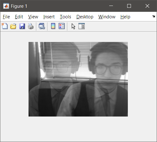
Great! Now we're ready to perform some real-time image processing. For fun, spend a few minutes devising an way to fake a long exposure...
Before we begin to look at Fourier decompositions, let's use a convolution through the function conv2 and measure the performance of our system as the kernel size increases.
rgb2gray() in your imshow() and snapsnot() functions to make our camera image grayscale.
tic and toc, estimate the frame rate of the system—the number of frames processed per second. Write this value out to the Command Window using disp() or equivalent. Remember that et = toc; will write the elapsed time in seconds to a variable.
conv2(). Pick five kernel sizes, and estimate the performance hit as the kernel size increases. Go big! Modern PCs are very fast, and we needed kernel sizes in the hundreds to see an impact. Keep the numbers handy. For more precise measurement in the real-time processing loop, take a running average of the framerate over a set of frames.
Fourier transforms are an important part of image processing which can be used to to decompose an image into a basis of sine and cosine components. In this lab, we will see some of the powers that Fourier transforms provide us when dealing with images.
In MATLAB, it is easy to compute Fourier transforms—we use the fft2() function. To compute the inverse of fourier transform, we can call ifft2(). The '2' here stands for '2D':
im = im2double( imread('rosso.png') );
im_f = fft2(im);
im_r = ifft2(im_f);
imshow( real(im_r) );


Let's investigate im_f. It is a complex double type, which means that it has both real and imaginary components (extractable with the real() and imag() functions, respectively). We saw in class what this means and how this is an elegant representation to the sine and cosine frequency basis via Euler's formula:
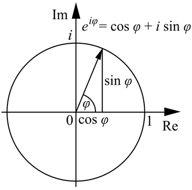
We also defined how these terms can be used to extract the frequency amplitude and phase components of the Fourier decomposition: $$A = \pm \sqrt{Re(\psi)^2+Im(\psi)^2}$$ $$\phi = \tan^{-1}( \frac{Im(\psi)}{Re(\psi)})$$
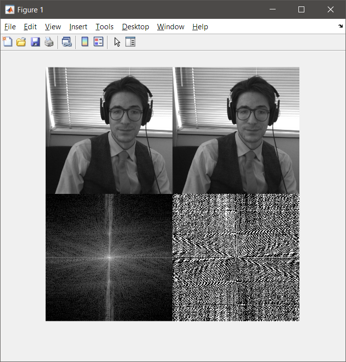
Let's look at the decomposition live. Adapt your live loop to also perform Fourier decoposition, and to visualize the input, frequency amplitude, phase, and reconstruction images.
im_f2 = re + 1j*im in MATLAB to return to the im_f complex double structure.
Some tips:
cat() liberally.
fftshift function to center the offset component (instead of it being at the edge of the image).
ifft2(), so that we can display it as an image.
Now that we have our decomposition in an easily manipulated format, let's edit it! We know that, in the frequency amplitude image, frequencies increase as we move out radially from the center, and horizontal and vertical frequencies lie on the y and x dimensions respectively. Please refer to the lecture slides for example editing operations.
By the convolution theorem of Fourier analysis, we know that convolution in the spatial domain is equivalent to element-wise multiplication of the frequency amplitude image in the frequency domain. This provides an opportunity: given that the computational cost of a Fourier decomposition is fixed, but that the computational cost of large kernel sizes increases (remember the first lab exercise), then we can use convolution in frequency space to speed up the execution of large kernels. MATLAB already does this for you if you use the imfilter() function, but not if you use the conv2().
conv2? At what kernel size does it become faster to convolve in the frequency domain than in the spatial domain?
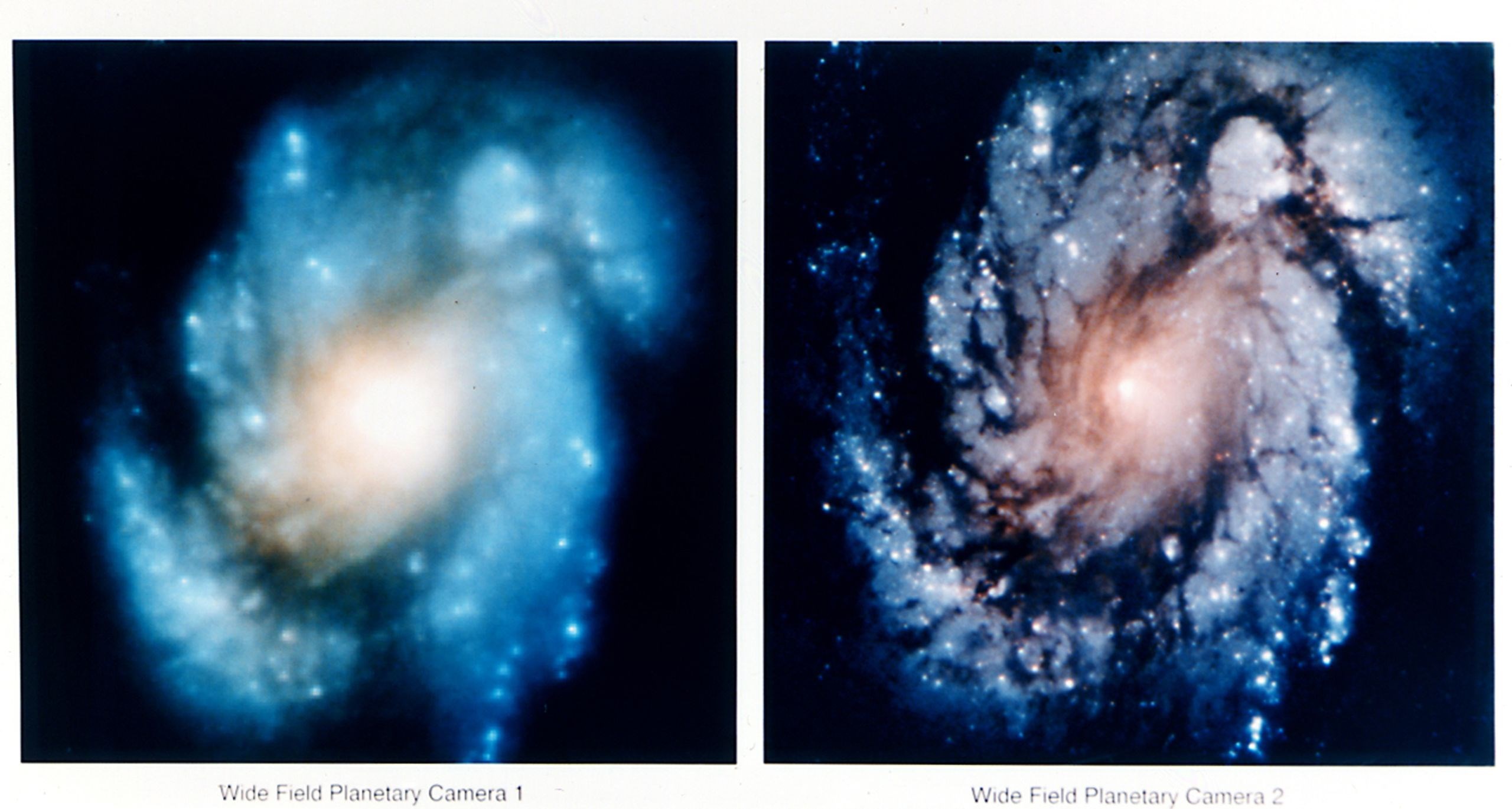
In class, we discussed that, by the convolution theorem, division in the Fourier domain is, in principle, a deblur or deconvolution. If we know the filter kernel, this deconvolution problem is possible (though the solution is unstable to even small amounts of noise). In most cases, we do not know the filter kernel and must estimate it. The Hubble Space Telescope's WFPC camera was famously blurry for the first three years of its operation due to an incorrectly-shaped mirror, but by imaging distant stars NASA could correct for and deconvolve Hubble's images.
Let's experiment with deconvolving given a known filter kernel.
Is deconvolution a well posed problem? How many possible scene and kernel combinations can make up a given image?
Important: When the values in the frequency amplitude channel of our Fourier decomposition are small (close to zero), this division causes problems as slight imprecision due to sampling noise causes large differences in output. Unfortunately, most point spread functions in imaging and optics have frequency decompositions with small amplitude values, which requires us to use strong regularization when deconvolving. This is beyond the scope of this lab, but interested parties can refer to Gordon Wetzstein's introduction here.
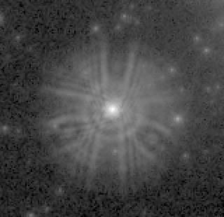
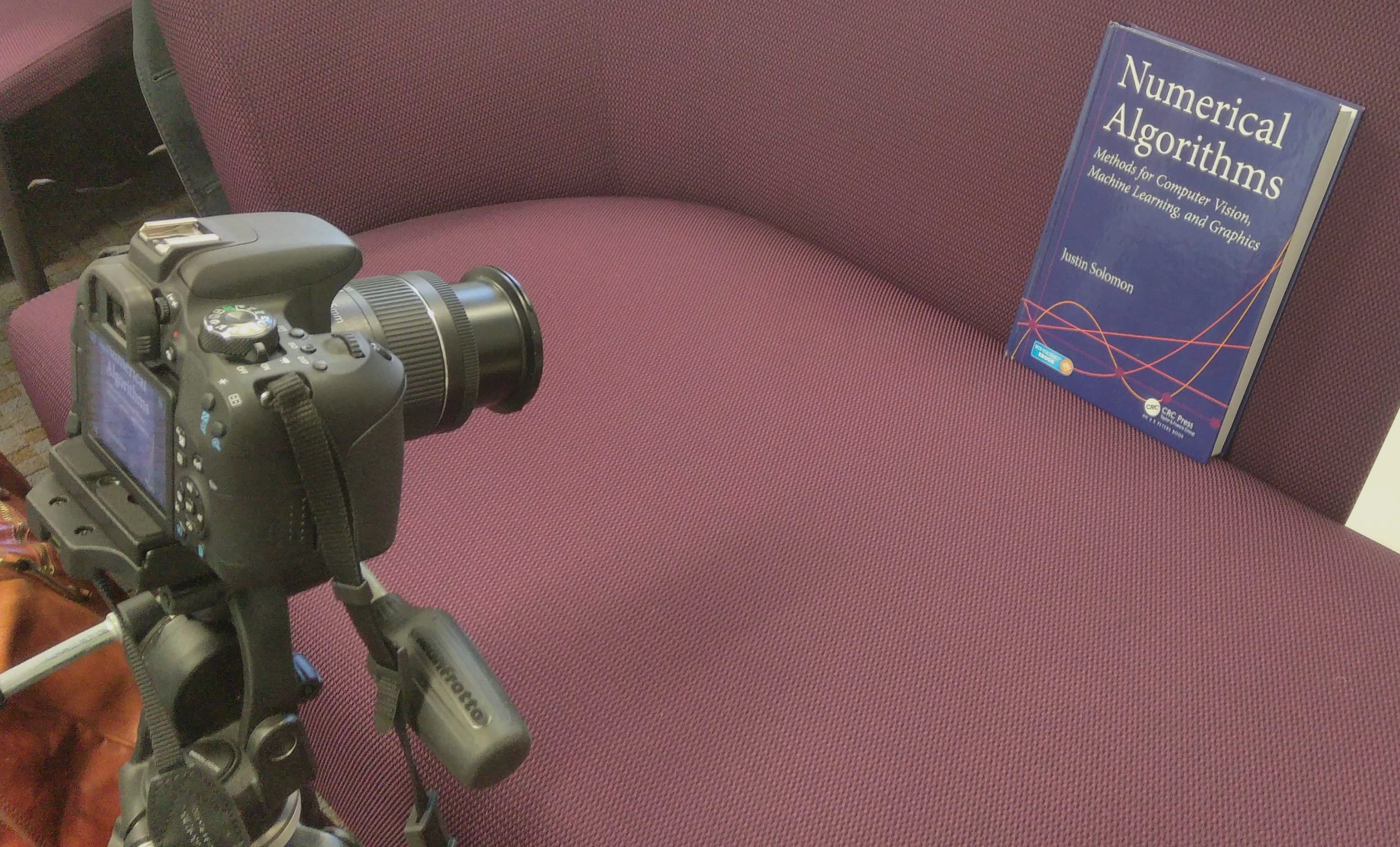
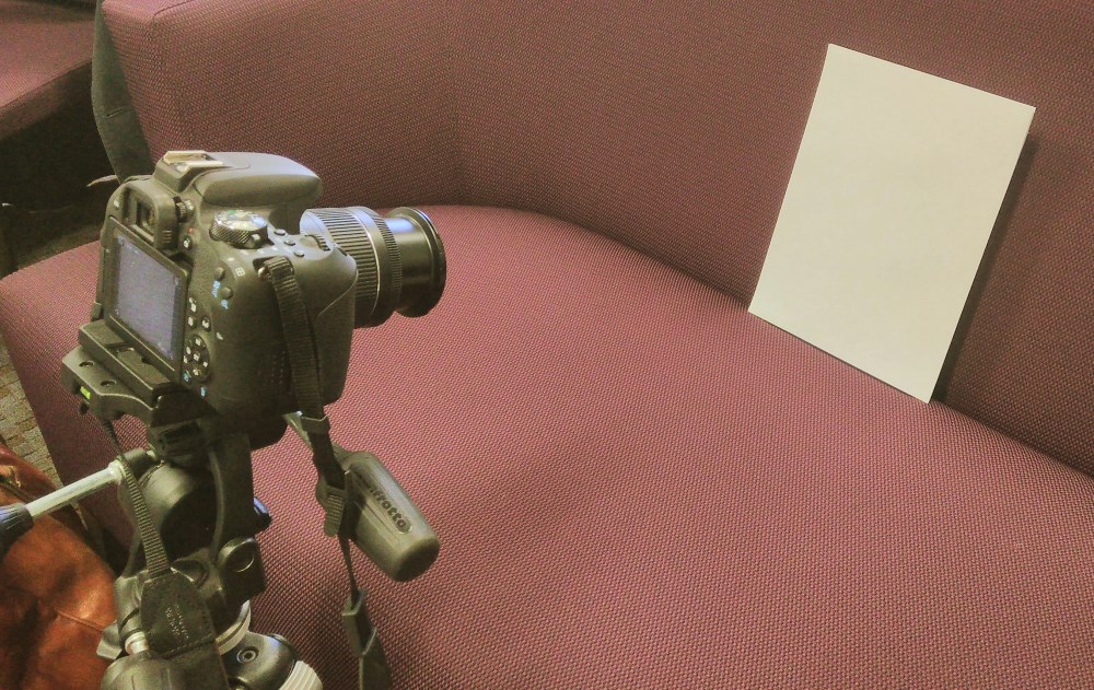
In real imaging applications, we usually don't know the kernel. How might we measure the optical blur (filter kernel) for a camera, to characterize depth of field and potentially deblur? One option is to image light from a single point in the world—a point light (or our best physical approximation of it)—and see how the light is spread across the sensor. This is called the point spread function (for obvious reasons). One way to image the point spread function is to photograph a single LED in a very dark room at a known distance away from the camera, and for known camera parameters (focal length, aperture). In principle, we can image the point spread function for all distances and all camera parameters, and calibrate or characterize the camera's depth of field blur. Then, if we knew the depth of a particular scene point in a new unseen photograph, we could deconvolve with the calibrated point spread function as a kernel.
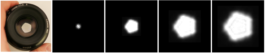
Phew! Seems hard (and laborious), but imagine performing this for just one depth and one set of camera parameters as an experiment, and then debluring an image of an object with planar geometry at that fixed depth. In principle, we could image any target that would allow us to measure the point spread function. It could be a point light, or we might try a tiny black dot on a smooth piece of paper or card (without any grain), which we could then invert.

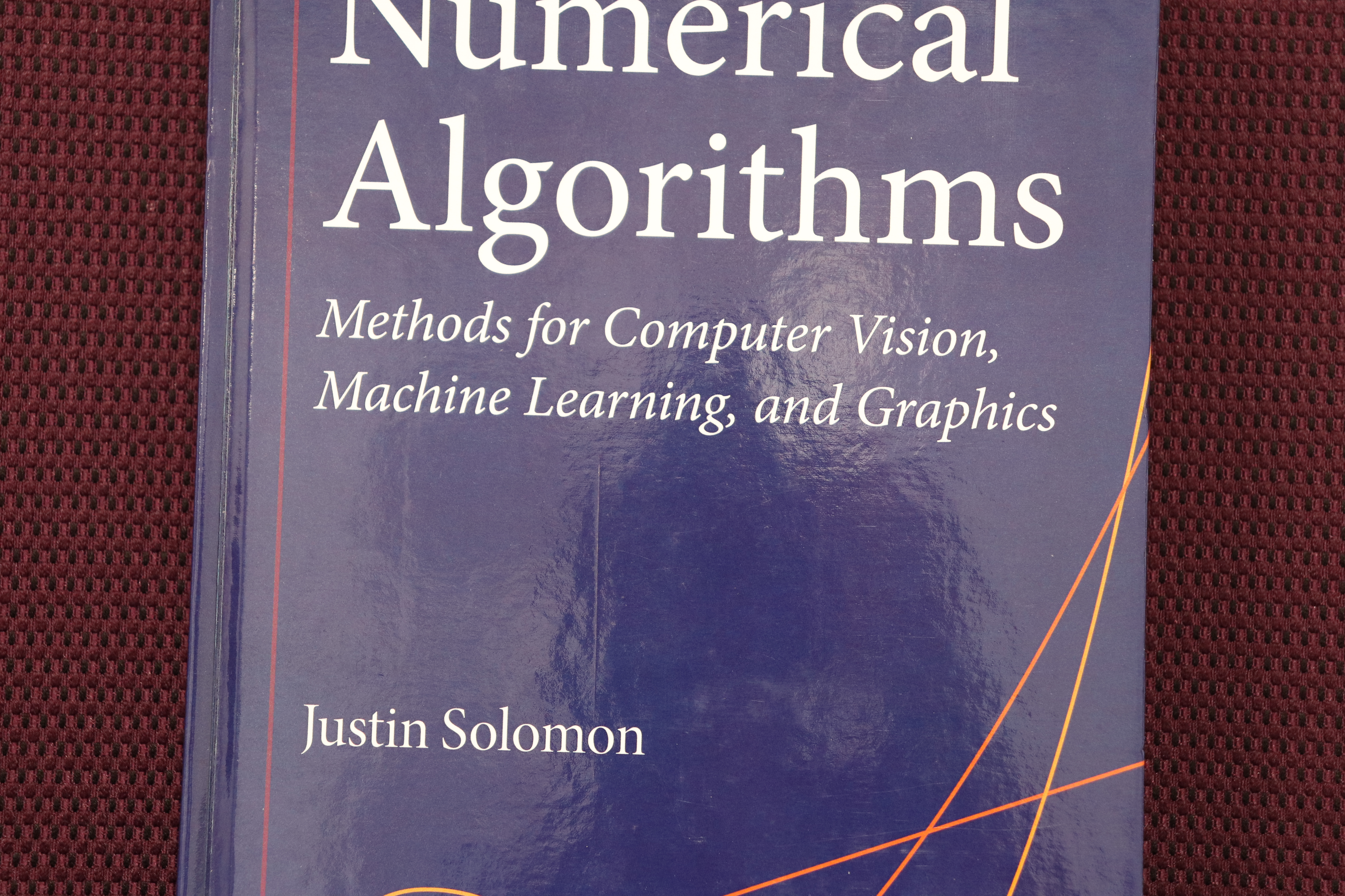
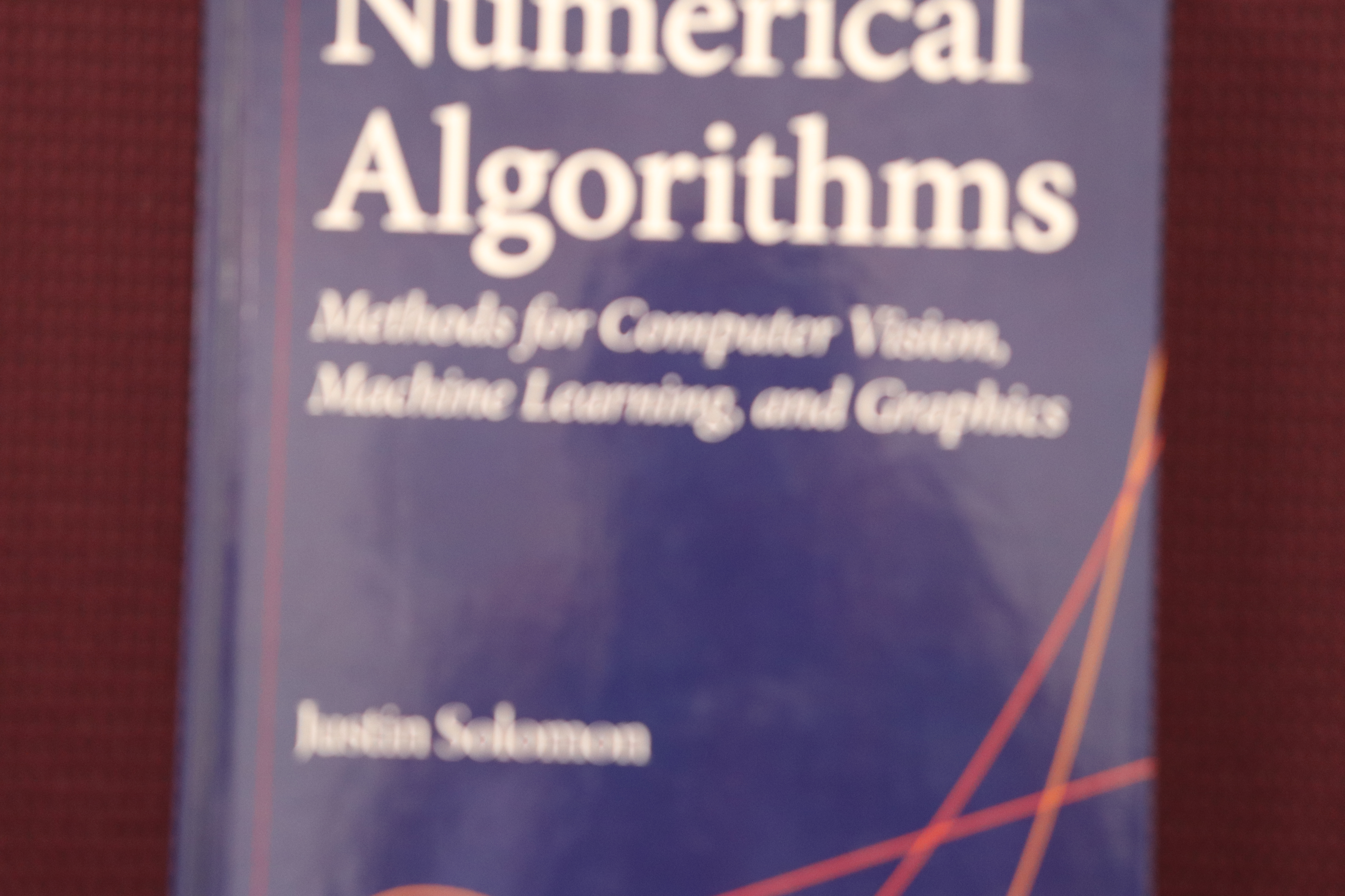
Would this approach work? What are the limitations of the approach? Is there a better workflow and computation?
Please upload your MATLAB code, input/result images, and any notes of interest as a PDF to Gradescope. Please use writeup.tex for your submission.
This lab was developed by Alan Yu and the 1290 course staff.