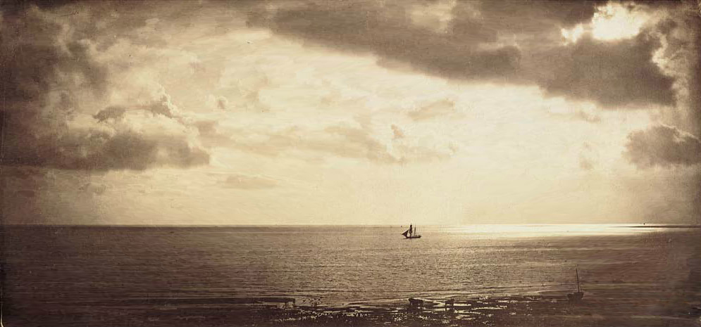
Gustave Le Gray arguably took the first high dynamic range images in the 1850s. Brig in the moonlight (retargeted above) was created via a manual process using seperate negatives for the sky and sea.

Project: High Dynamic Range

Logistics

• Files: Github Classroom
• Extra disk space: /course/cs1290_students
• Part 1: Questions
  • Questions + template in the zip: questions/
  • Hand-in process: Gradescope as PDF. Submit anonymous materials please!
  • Due: Weds 7th Oct. 2020, 9pm.
• Part 2: Code
  • Writeup template: In the zip: writeup/
  • Hand-in process: Gradescope. Upload your repo directly to Gradescope. There is an option to import a repo on submission.
  • If this fails: required files are in code/, writeup/writeup.pdf - use the createSubmissionZip.py script.
  • Submit anonymous materials please!
  • Due: Weds 14th Oct. 2020, 9pm.

Background

Modern cameras are unable to capture the full dynamic range of commonly encountered real-world scenes. In some scenes, even the best possible photograph will be partially under or over-exposed. Researchers and photographers commonly overcome this limitation by combining information from multiple exposures of the same scene. You will write software to automatically combine multiple exposures into a single high dynamic range radiance map, and then convert this radiance map to an image suitable for display through tone mapping.

Requirements

There are two major components to this project (plus writeup requirements):

1. +45 pts: Recovering a radiance map from a collection of images. You will have to recover the inverse of the function mapping exposure to pixel value, \(g\).
2. Converting this radiance map into an image suitable for viewing on a low dynamic range display:
   1. +10 pts: First, you will implement your favourite global tone mapping operator.
   2. +35 pts: Second, you will improve it by implementing a local tone mapping operator.
3. +10 pts: Write up
4. -5*n pts: Lose 5 points for every time (after the first) you do not follow the instructions for the hand in format

Stencil code note: Switching between image sets to perform radiance map recovery and tone mapping on is done through command line arguments. The lambda smoothing factor can also be manipulated this way. Run python3 main.py -h for more info.

Potentially useful functions: cv2.bilateralFilter() or equivalent.

Forbidden functions: cv2.createMergeDebevec() or equivalent; cv2.createTonemap() or equivalent.

Left: Recovered radiance map from shutter-time-varying exposures.
Right: Tone mapped result with global operator from Reinhard et al.

Write up

Complete the following:

1. Visualize your radiance maps (the stencil code will write out your images to disk).
2. Plot the graph of the recovered relationship between exposure and pixel values, both without and with the second-derivative smoothing term and tent function weighting.
3. Show the bilateral filtering based decomposition into low and high frequency image components.
4. Show tonemapping results for all test cases, compared against baselines such as linear dynamic range compression or the Reinhard et al. global operator.

In addition to all of this, please describe your process and algorithm, describe any extra credit and show its effect, tell us any other information you feel is relevant, and cite your sources. We provide you with a LaTeX template in writeup/writeup.tex. Please compile it into a PDF and submit it along with your code. In class, we will present the project results for interesting cases.

Task: Submit writeup/writeup.pdf

We conduct anonymous TA grading, so please don't include your name or ID in your writeup or code.

Extra Credit

• up to 3 points: Try the algorithm on your own photos!
• up to 3 points: Try your tone mapping algorithms on an already-linear RAW image from a camera with a more sensitive sensor (e.g., the class' 14-bit Canon T7i cameras), and compare it to your HDR reconstruction from your smartphone camera (perhaps also the 'HDR' mode from your camera app).
• Some of the test image stacks are not well aligned (e.g., garden). Try to automatically correct the geometric alignment of the images before running your HDR pipeline.
  • up to 3 points: For implementations similar to Project 1.
  • up to 5 points: For local alignment methods.
• up to 10 points: Implement any other local tone mapping algorithm. For example a "simplified version" of this algorithm.
• up to 10 points: Implement the fast bilateral filtering optimization described here (thanks to Sylvain Paris) in which Gaussian convolutions are performed in a subsampled 3d space. Discuss the speedup achieved over the baseline method.
• up to 10 points: Implement Exposure Fusion by Mertens et al., which is a simple way to create a cross-exposure image without needing HDR at all. See lecture slides at end of the 1290 deck on HDR.

For all extra credit, be sure to demonstrate in your write up cases where your extra credit has improved image quality or computation speed.

Hand in

You will lose points if you do not follow instructions. Every time after the first that you do not follow instructions, you will lose 5 points. The folder you hand in must contain the following:

• code/ - directory containing all your code for this assignment
• writeup/writeup.pdf - your report as a PDF file generated with Latex.

Use Gradescope to submit your repo directly. When creating a subission, you will be asked to upload your repo. In this project, you should be able to commit images to the repo and submit through Gradescope. Make sure only the necessary images for your handin are included.

Implementation Details

Literature

The two relevant papers are Debevec and Malik 1997 and Durand 2002. We will reference them in the description below.

Radiance map reconstruction

We want to reconstruct an HDR radiance map from several LDR exposures. It is highly recommended that you read Sections 2.1 and 2.2 in Debevec and Malik 1997 to help understand this process. There are also slides in the HDR deck (not shown in class) which detail this process. Below is a summary.

The observed pixel value \(Z_{ij}\) for pixel \(i\) in image \(j\) is a function of unknown scene radiance and known exposure duration: $$Z_{ij} = f(E_i \Delta t_j ).$$ \(E_i\) is the unknown scene radiance at pixel \(i\), and integrating scene radiance over some time \(E_i \Delta t_j\) is the exposure at a given pixel. In general, \(f\) might be a somewhat complicated pixel response curve. We will not solve for \(f\), but for \(g = ln(f^{-1})\) which maps from pixel values (from \(0\) to \(255\)) to the log of exposure values (Equation 2 in Debevec and Malik): $$g(Z_{ij}) = ln(E_i) + ln(t_j).$$ Solving for \(g\) might seem impossible (and indeed, we only recover \(g\) up to a scale factor) because we know neither \(g\) or \(E_i\). The key observation is that the scene is static, and while we might not know the absolute value of \(E_i\) at each pixel \(i\), we do know that the scene radiance remains constant across the image sequence.

Solving for \(g\) is the tricky part. After we have \(g\), is it straightforward to map from the observed pixels values and shutter times to radiance by the following equation (rearranged from above): $$ln(E_i) = g(Z_{ij}) - ln(\Delta t_j).$$ This is Equation 5 in Debevec.

To make the results robust, we want to consider two additional things:

• Second-derivative smoothing term: We expect \(g\) to be smooth. Debevec adds a constraint to our linear system which penalizes \(g\) according to the magnitude of its second derivative. Since \(g\) is discrete (defined only at integer values from \(g(0)\) to \(g(255)\) we can approximate the second derivative with finite differences, e.g.: $$g''(x) = (g(x-1) - g(x)) - (g(x) - g(x+1)) = g(x-1) + g(x+1) - 2g(x).$$ We will have one such equation for each integer in the domain of \(g\), except for \(g(0)\) and \(g(255)\) where the second derivative would be undefined.
• Tent function weighting: Each exposure only gives us trustworthy information about certain pixels (i.e., the well exposed pixels for that image). For dark pixels the relative contribution of noise is high and for bright pixels the sensor may have been saturated. To make our estimates of \(E_i\) more accurate, we need to weight the contribution of each pixel according to Equation 6 in Debevec. An example of a weighting function \(w\) is a triangle function that peaks at \(Z=127.5\), and is zero at \(Z=0\) and \(Z=255\). This is provided for you in the starter code. This weighting should be used both when solving for \(g\) and when using \(g\) to build the HDR radiance map for all pixels.

Tone mapping

Recovering the radiance map is only half the battle—we wish to show detail in dark and bright image regions on a low-dynamic-range display. There are a few gobal tone-mapping operators to play with, such as \(\log(E)\), \(\sqrt{E}\), and \(E / (1+E)\) (the Reinhard et al. operator). Regardless of which transform we use, we wish to stretch the intensity values in the resulting image to fill the [0 255] range for maximum contrast.

Once you see something reasonable using a global tone mapping operation, we wish to implement a local method for full credit.

We will implement a simplified version of Durand 2002. The steps are roughly as follows:

1. Input is linear RGB values of radiance.
2. Compute the average intensity \(I\) by averaging the color channels per pixel of the output radiance map.
3. Compute the chrominance channels: \(R/I, G/I, B/I\)
4. Compute the log intensity: \(E = \log_2(I)\)
5. Filter that with a bilateral filter to produce the `large scale' intensity: \(B = bf(E)\)
6. Compute the detail layer: \(D = E - B\)
7. Apply an offset and a scale to the base: \(B' = (B - o) * s\)
   1. The offset is such that the maximum intensity of the base is \(1\). Since the values are in the log domain, \(o = max(B)\).
   2. The scale is set so that the output base has dR stops of dynamic range, i.e., \(s = dR / (max(B) - min(B))\). Try values between 2 and 8 for \(dR\), that should cover an interesting range. Values around 4 or 5 should look fine.
8. Reconstruct the log intensity: \(O = 2^{(B' + D)}\)
9. Put back the colors: \(R',G',B' = O * (R/I, G/I, B/I)\)
10. Apply gamma compression. Without gamma compression the result will look too dark. Values around 0.5 should look fine (e.g., result.^0.5). You can also apply the simple global intensity scaling to your final output.

Tips

• Images in the ./data/ directory are named for their exposure in seconds as a fraction, where underscore separates the nominator from the denominator.
• To create results which are clearly better than any single exposure, make sure your scene actually has a high dynamic range! The data we give you have combinations of very bright (sunlight or bright lights) and very dark (shadowed) elements. If you take your own photos, take photos that have combinations of indoor and outdoor elements, or scenes that are heavily back-lit, possibly with the light source directly visible.
• MATLAB code for recovering \(g\) is available in Debevec and Malik 1997 and in the lecture slides in class. You can look at this as a reference.
• Your HDR images have zero values which will cause problems with \(log\). You can fix this problem by replacing all zeros by some factor times the smallest non-zero values.
• The bilateral filter is sensitive to the sigma values for the intensity Gaussian and spatial Gaussian. The spatial component of the bilateral filter should have a large spatial extent.
• For your own photos, and for any photos with long exposures, geometric alignment to correct for camera motion will probably improve your results.

Acknowledgements

Project partially based on Noah Snavely's Computer Vision course at Cornell University, with permission. Handout written by David Dufresne, Travis Webb, Sam Birch, Emanuel Zgraggen, and James Hays. Conversion to Python from MATLAB by Isa Milefchik.

Outline of Durand 2002 provided by Sylvain Paris.

Some of the test images have been taken from:
http://www.cs.brown.edu/courses/csci1950-g/results/final/dkendall/
http://www.pauldebevec.com/Research/HDR/
http://cybertron.cg.tu-berlin.de/eitz/